
Unique Paths III - Solution & Explanation
Problem Statement
You are given an m x n integer array grid where grid[i][j] could be:
1representing the starting square. There is exactly one starting square.2representing the ending square. There is exactly one ending square.0representing empty squares we can walk over.-1representing obstacles that we cannot walk over.
Return the number of 4-directional walks from the starting square to the ending square, that walk over every non-obstacle square exactly once.
Example 1:

Input: grid = [[1,0,0,0],[0,0,0,0],[0,0,2,-1]]
Output: 2
Explanation: We have the following two paths:
1. (0,0),(0,1),(0,2),(0,3),(1,3),(1,2),(1,1),(1,0),(2,0),(2,1),(2,2)
2. (0,0),(1,0),(2,0),(2,1),(1,1),(0,1),(0,2),(0,3),(1,3),(1,2),(2,2)
Example 2:
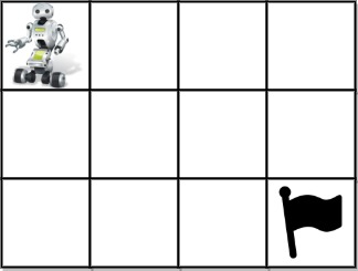
Input: grid = [[1,0,0,0],[0,0,0,0],[0,0,0,2]]
Output: 4
Explanation: We have the following four paths:
1. (0,0),(0,1),(0,2),(0,3),(1,3),(1,2),(1,1),(1,0),(2,0),(2,1),(2,2),(2,3)
2. (0,0),(0,1),(1,1),(1,0),(2,0),(2,1),(2,2),(1,2),(0,2),(0,3),(1,3),(2,3)
3. (0,0),(1,0),(2,0),(2,1),(2,2),(1,2),(1,1),(0,1),(0,2),(0,3),(1,3),(2,3)
4. (0,0),(1,0),(2,0),(2,1),(1,1),(0,1),(0,2),(0,3),(1,3),(1,2),(2,2),(2,3)
Example 3:
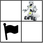
Input: grid = [[0,1],[2,0]]
Output: 0
Explanation: There is no path that walks over every empty square exactly once.
Note that the starting and ending square can be anywhere in the grid.
Constraints:
m == grid.lengthn == grid[i].length1 <= m, n <= 201 <= m * n <= 20-1 <= grid[i][j] <= 2- There is exactly one starting cell and one ending cell.
Approach Overview
Problem Overview: You are given a grid containing a start cell, an end cell, empty squares, and obstacles. Count how many paths move from start to end while visiting every non-obstacle cell exactly once. Movement is allowed in four directions, and you cannot revisit a cell.
Approach 1: Backtracking with Depth-First Search (O(3^k) time, O(k) space)
This problem naturally maps to backtracking over a matrix. First scan the grid to locate the start position and count how many cells must be visited (all empty cells plus the start). From the start, run DFS and recursively explore four directions. Mark the current cell as visited (often by temporarily modifying the grid), decrement the remaining cell counter, and continue exploring neighbors that are inside bounds and not obstacles. When you reach the end cell, the path is valid only if every required cell has been visited.
The key insight: each recursive call represents a partial path. Backtracking restores the cell state after exploring a branch so other paths can reuse it. Since you can move to at most three new cells at each step (excluding the previous cell), the search space is roughly O(3^k), where k is the number of walkable cells. Space complexity is O(k) due to the recursion stack. This approach is straightforward and performs well because grid sizes are small.
Approach 2: Dynamic Programming with State Compression (O((m*n) * 2^k) time, O((m*n) * 2^k) space)
This approach models the problem as visiting cells with a bitmask representing the visited state. Each walkable cell receives an index. A DP state looks like dp[r][c][mask], meaning the number of ways to reach cell (r,c) with the set of visited cells encoded in mask. Transition by moving to adjacent cells and updating the bitmask using bit manipulation. The final answer counts states where the end cell is reached with every required bit set.
The insight is that path validity depends only on the current position and which cells were already visited. Encoding visited cells as a bitmask avoids recomputation of identical states encountered via different paths. With k walkable cells, there are at most 2^k masks and m*n positions, producing O((m*n) * 2^k) states. Although heavier in memory, this method demonstrates how Hamiltonian path-style grid problems can be solved using state compression.
Recommended for interviews: Backtracking with DFS is the expected solution. It directly models the constraint of visiting every square exactly once and is easier to implement under pressure. Interviewers often look for clean recursion, correct base conditions, and proper state restoration. State compression DP is an advanced optimization idea and useful when discussing alternative formulations or demonstrating strong understanding of bitmask DP.
Approach 1: Backtracking with Depth-First Search
This approach uses a Depth-First Search (DFS) technique with backtracking to explore every possible path from the start to the end square. We first count all the empty squares and ensure that each path covers all these squares exactly once. Starting from the initial position, we recursively visit adjacent squares, marking them as visited to ensure they aren't visited again during the same path. If a path reaches the end square and has visited all empty squares, it's a valid path.
The solution uses DFS to explore all possible paths recursively. The dfs() function is defined to attempt moving in four directions from the current cell. We mark the current cell as visited by temporarily setting it to -2 and backtrack by restoring its value to 0, enabling alternative paths. We use a counter variable, remain, to track the number of unvisited non-obstacle squares. If we reach the target square after visiting all non-obstacle squares, it's counted as one unique path.
Complexity
Time Complexity: O(3^(m*n)). In the worst case, we explore each cell in multiple directions.
Space Complexity: O(m*n), due to recursion stack.
Approach 2: Dynamic Programming with State Compression
In this approach, we use dynamic programming to reduce the problem into smaller overlapping subproblems. With state compression, we leverage bitmasking to track visited squares in the grid efficiently. Each state is represented by a combination of the current cell and a bitmask that indicates which of the necessary cells (squares) have been covered. The problem then simplifies into finding paths to cover large subproblems using previously computed smaller subproblem solutions.
This method involves initializing a 2D DP table and iteratively computing the number of paths by considering smaller subsets of the grid using bitmask representation. Each cell represents the state of paths leading to it, which can be updated from adjacent cells. This method maximizes efficiency by avoiding repetitive computations, combining overlapping solutions with dynamic programming. Details are omitted due to space limitations.
Code
Python
Complexity
Time Complexity: O(m * n * 2^{mn}), based on distinct achievable states across board size.
Space Complexity: O(m * n * 2^{mn}), attributed to DP table size.
Approach 3: Backtracking
We can first traverse the entire grid, find the starting point (x, y), and count the number of blank spaces cnt.
Next, we can start searching from the starting point to get all the path numbers. We design a function dfs(i, j, k) to indicate that the path number is k and the starting point is (i, j).
In the function, we first determine whether the current cell is the end point. If it is, we determine whether k is equal to cnt + 1. If it is, the current path is a valid path, and 1 is returned, otherwise 0 is returned.
If the current cell is not the end point, we enumerate the four adjacent cells of the current cell. If the adjacent cell has not been visited, we mark the adjacent cell as visited, and then continue to search the path number from the adjacent cell. After the search is completed, we mark the adjacent cell as unvisited. After the search is completed, we return the sum of the path numbers of all adjacent cells.
Finally, we return the path number from the starting point, that is, dfs(x, y, 1).
The time complexity is O(3^{m times n}), and the space complexity is O(m times n). Where m and n are the number of rows and columns of the grid, respectively.
Code
Python
Java
C++
Go
TypeScript
JavaScript
Complexity Comparison
| Approach | Complexity |
|---|---|
| Backtracking with Depth-First Search | Time Complexity: O(3^(m*n)). In the worst case, we explore each cell in multiple directions. |
| Dynamic Programming with State Compression | Time Complexity: O(m * n * 2^{mn}), based on distinct achievable states across board size. |
| Backtracking | — |
Detailed Complexity Analysis
| Approach | Time | Space | When to Use |
|---|---|---|---|
| Backtracking with Depth-First Search | O(3^k) | O(k) | Best practical solution for the problem. Grid sizes are small and DFS cleanly enumerates all valid paths. |
| Dynamic Programming with State Compression | O((m*n) * 2^k) | O((m*n) * 2^k) | Useful when exploring Hamiltonian path style problems or demonstrating bitmask DP techniques. |
Video Solution
Unique Paths III -(Apple, Amazon, Microsoft, Intuit) : Explanation ➕ Live Coding • codestorywithMIK • 21,017 views views
Watch 9 more video solutions →Frequently Asked Questions
Is Unique Paths III easy or hard?
How to solve Unique Paths III in O(n)?
What is the best approach for Unique Paths III?
What data structure is used in Unique Paths III?
What is the time complexity of Unique Paths III?
Unique Paths III Python or Java solution approach?
Is Unique Paths III asked at Google, Amazon, or Meta?
Ready to solve this problem?
Practice Unique Paths III with our built-in code editor and test cases.
Practice on FleetCodeProblem Info
Table of Contents
Practice this problem
Open in Editor