You are in a city that consists of n intersections numbered from 0 to n - 1 with bi-directional roads between some intersections. The inputs are generated such that you can reach any intersection from any other intersection and that there is at most one road between any two intersections.
You are given an integer n and a 2D integer array roads where roads[i] = [ui, vi, timei] means that there is a road between intersections ui and vi that takes timei minutes to travel. You want to know in how many ways you can travel from intersection 0 to intersection n - 1 in the shortest amount of time.
Return the number of ways you can arrive at your destination in the shortest amount of time. Since the answer may be large, return it modulo 109 + 7.
Example 1:
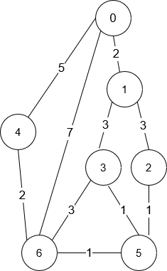
Input: n = 7, roads = [[0,6,7],[0,1,2],[1,2,3],[1,3,3],[6,3,3],[3,5,1],[6,5,1],[2,5,1],[0,4,5],[4,6,2]]
Output: 4
Explanation: The shortest amount of time it takes to go from intersection 0 to intersection 6 is 7 minutes.
The four ways to get there in 7 minutes are:
- 0 ➝ 6
- 0 ➝ 4 ➝ 6
- 0 ➝ 1 ➝ 2 ➝ 5 ➝ 6
- 0 ➝ 1 ➝ 3 ➝ 5 ➝ 6
Example 2:
Input: n = 2, roads = [[1,0,10]]
Output: 1
Explanation: There is only one way to go from intersection 0 to intersection 1, and it takes 10 minutes.
Constraints:
1 <= n <= 200n - 1 <= roads.length <= n * (n - 1) / 2roads[i].length == 30 <= ui, vi <= n - 11 <= timei <= 109ui != viProblem Overview: Given n intersections and bidirectional roads with travel times, compute how many distinct ways you can reach node n-1 from node 0 using the minimum total time. The graph can contain multiple routes, but only paths with the shortest distance count. The result must be returned modulo 1e9 + 7.
Approach 1: Dijkstra's Algorithm with Path Counting (Time: O(E log V), Space: O(V + E))
This approach combines classic shortest path computation with dynamic counting of paths. Use an adjacency list and a min-heap priority queue to run Dijkstra from node 0. Maintain two arrays: dist[i] for the shortest distance to node i, and ways[i] for the number of shortest paths reaching that node. When relaxing an edge, update normally if a strictly shorter distance is found and copy the path count from the parent. If another path reaches the same node with the exact same shortest distance, add the parent’s path count instead of replacing it. This effectively layers a dynamic programming idea on top of Dijkstra. The priority queue ensures nodes are processed in increasing distance order, which guarantees correctness for weighted graphs with non‑negative edges.
Approach 2: Bellman-Ford Adaptation (Time: O(V * E), Space: O(V))
Another way to compute shortest paths is the Bellman-Ford relaxation process. Iterate over all edges up to V-1 times, updating distances similarly to standard Bellman-Ford. Alongside the distance array, track a ways[] array storing the number of shortest routes to each node. When a relaxation produces a smaller distance, copy the path count from the source node; when it produces the same distance, add the counts. This approach works even if the algorithm repeatedly revisits nodes because the relaxations converge toward the minimum distance. The drawback is performance: iterating over every edge for each pass makes it significantly slower than heap-based methods for dense graphs.
Recommended for interviews: The expected solution uses Dijkstra with path counting. Interviewers want to see that you recognize the problem as a weighted graph shortest-path problem and augment the algorithm to track the number of optimal routes. Starting from brute reasoning about shortest paths is fine, but implementing the heap-based solution demonstrates strong algorithmic intuition and efficient handling of weighted graphs.
Description: This approach extends the classic Dijkstra's algorithm by integrating path counting. During the process of finding the shortest path using Dijkstra's algorithm, we will maintain an additional array to count the number of ways to reach each node in the graph in the shortest time.
Steps:
Considerations: Ensure counting is done modulo 109 + 7 to handle large numbers.
This Python function utilizes Dijkstra's algorithm via a min-heap (priority queue) to compute the shortest travel time. It adds functionality to track the number of shortest paths leading to each node. Each time a node is visited, if a shorter path is found, it updates; if equally short, it increments the path count using modular arithmetic.
Python
JavaScript
Time Complexity: O((N + E) log N), where N is the number of nodes and E is the number of edges.
Space Complexity: O(N + E) for the graph representation and additional arrays.
Description: An adaptation of the Bellman-Ford algorithm is possible here due to its suitability for graphs with non-negative weights, though less efficient, still valid for counting shortest paths under simple constraints.
Steps:
Note: Though not the most optimized under standard constraints as seen with Dijkstra's, exploring this aids learning.
The Java solution employs Bellman-Ford to establish shortest paths by iteratively relaxing all edges. Additional logic manages path counting upon equal length paths. Repeated edge checks across (n-1) rounds ensure comprehension of total optimal paths.
Time Complexity: O(N * E), given every edge relaxes across nodes.
Space Complexity: O(N) for maintaining distances and counts arrays.
We define the following arrays:
g represents the adjacency matrix of the graph. g[i][j] represents the shortest path length from point i to point j. Initially, all are infinity, while g[0][0] is 0. Then we traverse roads and update g[u][v] and g[v][u] to t.dist[i] represents the shortest path length from the starting point to point i. Initially, all are infinity, while dist[0] is 0.f[i] represents the number of shortest paths from the starting point to point i. Initially, all are 0, while f[0] is 1.vis[i] represents whether point i has been visited. Initially, all are False.Then, we use the naive Dijkstra algorithm to find the shortest path length from the starting point to the end point, and record the number of shortest paths for each point during the process.
Finally, we return f[n - 1]. Since the answer may be very large, we need to take the modulus of 10^9 + 7.
The time complexity is O(n^2), and the space complexity is O(n^2), where n is the number of points.
Python
Java
C++
Go
TypeScript
| Approach | Complexity |
|---|---|
| Dijkstra's Algorithm with Path Counting | Time Complexity: O((N + E) log N), where N is the number of nodes and E is the number of edges. |
| Bellman-Ford Algorithm Adaptation | Time Complexity: O(N * E), given every edge relaxes across nodes. |
| Naive Dijkstra Algorithm | — |
| Approach | Time | Space | When to Use |
|---|---|---|---|
| Dijkstra's Algorithm with Path Counting | O(E log V) | O(V + E) | Best choice for weighted graphs with non-negative edges. Efficient and commonly expected in interviews. |
| Bellman-Ford Adaptation | O(V * E) | O(V) | Useful when demonstrating relaxation-based shortest path logic or when negative edges are possible. |
G-40. Number of Ways to Arrive at Destination • take U forward • 222,170 views views
Watch 9 more video solutions →Practice Number of Ways to Arrive at Destination with our built-in code editor and test cases.
Practice on FleetCode