A city is represented as a bi-directional connected graph with n vertices where each vertex is labeled from 1 to n (inclusive). The edges in the graph are represented as a 2D integer array edges, where each edges[i] = [ui, vi] denotes a bi-directional edge between vertex ui and vertex vi. Every vertex pair is connected by at most one edge, and no vertex has an edge to itself. The time taken to traverse any edge is time minutes.
Each vertex has a traffic signal which changes its color from green to red and vice versa every change minutes. All signals change at the same time. You can enter a vertex at any time, but can leave a vertex only when the signal is green. You cannot wait at a vertex if the signal is green.
The second minimum value is defined as the smallest value strictly larger than the minimum value.
[2, 3, 4] is 3, and the second minimum value of [2, 2, 4] is 4.Given n, edges, time, and change, return the second minimum time it will take to go from vertex 1 to vertex n.
Notes:
1 and n.
Example 1:
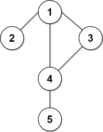
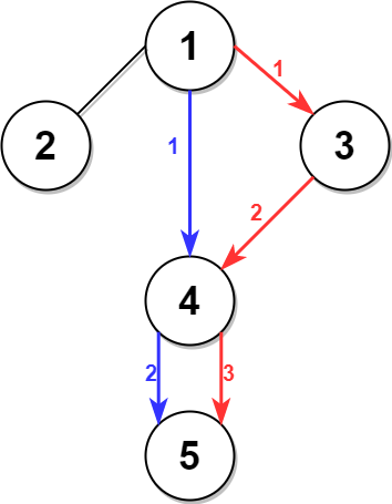
Input: n = 5, edges = [[1,2],[1,3],[1,4],[3,4],[4,5]], time = 3, change = 5
Output: 13
Explanation:
The figure on the left shows the given graph.
The blue path in the figure on the right is the minimum time path.
The time taken is:
- Start at 1, time elapsed=0
- 1 -> 4: 3 minutes, time elapsed=3
- 4 -> 5: 3 minutes, time elapsed=6
Hence the minimum time needed is 6 minutes.

The red path shows the path to get the second minimum time.
- Start at 1, time elapsed=0
- 1 -> 3: 3 minutes, time elapsed=3
- 3 -> 4: 3 minutes, time elapsed=6
- Wait at 4 for 4 minutes, time elapsed=10
- 4 -> 5: 3 minutes, time elapsed=13
Hence the second minimum time is 13 minutes.
Example 2:

Input: n = 2, edges = [[1,2]], time = 3, change = 2
Output: 11
Explanation:
The minimum time path is 1 -> 2 with time = 3 minutes.
The second minimum time path is 1 -> 2 -> 1 -> 2 with time = 11 minutes.
Constraints:
2 <= n <= 104n - 1 <= edges.length <= min(2 * 104, n * (n - 1) / 2)edges[i].length == 21 <= ui, vi <= nui != vi1 <= time, change <= 103Problem Overview: You are given an undirected graph where each edge takes the same travel time, but intersections have traffic signals that alternate between green and red every change minutes. The goal is to reach node n from node 1, not with the shortest travel time, but with the second minimum arrival time while respecting signal delays.
Approach 1: Breadth-First Search with Traffic Signal Simulation (Time: O(E), Space: O(V))
This approach uses Breadth-First Search on the graph while tracking the first and second arrival times for every node. Instead of storing only one distance, maintain two values: the shortest and second shortest arrival time. Each time you move along an edge, compute whether you must wait for the signal. If the current time falls in a red phase ((time / change) % 2 == 1), wait until the next green phase before traveling. Push new arrival times into the BFS queue only if they improve the first or second best time for that node. The algorithm stops once the second arrival time for node n is discovered.
The key insight is that BFS works because all edges have equal traversal time. The additional logic handles signal waiting and ensures each node records up to two unique arrival times.
Approach 2: Modified Dijkstra's Algorithm (Time: O(E log V), Space: O(V))
This method models the problem as a shortest path search where each node can be visited twice with different arrival times. Use a priority queue to always expand the smallest current time. When exploring neighbors, calculate the departure time considering signal cycles: if the light is red, wait until the next green interval before adding edge travel time. Maintain two best arrival times per node and ignore any candidate that is not among the top two.
The modified Dijkstra structure guarantees correct ordering of times, which simplifies reasoning about when the second minimum path is finalized. It works well when you want strict ordering of states and deterministic expansion of earliest arrival times.
Recommended for interviews: The BFS-based solution is usually preferred because all edges have equal weight. Interviewers expect you to recognize that this is a graph traversal problem with multiple valid distances per node. Showing the two-distance tracking technique demonstrates strong understanding of BFS and shortest-path variations, while the Dijkstra variant proves you can generalize the idea when edge weights or timing rules become more complex.
This approach involves using a priority queue to simulate a modified version of Dijkstra's algorithm, aiming to track both the shortest and second shortest path times to the last node. The cost of each step is affected by traffic signal delays, calculated based on the cumulative time spent traveling.
This solution builds a graph using an adjacency list. We use a priority queue to explore paths encapsulated by their current time and destination node. For each node, we maintain two arrays to keep track of the first and second minimum time taken to reach it. The algorithm updates these values by considering wait times if a traffic light is red. We return the second minimum time to reach the destination node.
The time complexity is O(E log V), where E is the number of edges, and V is the number of vertices, due to the priority queue operations. The space complexity is O(V + E) due to the storage of the adjacency list and the min_time/second_min_time arrays.
This approach leverages a Breadth-First Search (BFS) to explore paths in level order, carefully managing path times with respect to traffic signal cycles. Time values are stored to identify both the shortest and second shortest paths throughout the search.
This JavaScript solution employs BFS with time management using traffic signal states to uncover the minimum and second minimum path costs. Paths are explored level by level, with state transitions manipulated using queue operations.
JavaScript
C#
C++
The time complexity is O(E) due to the traversal of all edges and the space complexity is O(V + E) for graph and time-tracking arrays.
| Approach | Complexity |
|---|---|
| Modified Dijkstra's Algorithm | The time complexity is O(E log V), where E is the number of edges, and V is the number of vertices, due to the priority queue operations. The space complexity is O(V + E) due to the storage of the adjacency list and the min_time/second_min_time arrays. |
| Breadth-First Search with Traffic Signal Consideration | The time complexity is O(E) due to the traversal of all edges and the space complexity is O(V + E) for graph and time-tracking arrays. |
| Default Approach | — |
| Approach | Time | Space | When to Use |
|---|---|---|---|
| Breadth-First Search with Signal Simulation | O(E) | O(V) | Best when all edges have equal travel time and you only need the first and second arrival times. |
| Modified Dijkstra's Algorithm | O(E log V) | O(V) | Useful when reasoning about ordered arrival times or when extending to weighted edges. |
Second Minimum Time to Reach Destination - Leetcode 2045 - Python • NeetCodeIO • 12,195 views views
Watch 9 more video solutions →Practice Second Minimum Time to Reach Destination with our built-in code editor and test cases.
Practice on FleetCodePractice this problem
Open in Editor