Given an undirected tree consisting of n vertices numbered from 1 to n. A frog starts jumping from vertex 1. In one second, the frog jumps from its current vertex to another unvisited vertex if they are directly connected. The frog can not jump back to a visited vertex. In case the frog can jump to several vertices, it jumps randomly to one of them with the same probability. Otherwise, when the frog can not jump to any unvisited vertex, it jumps forever on the same vertex.
The edges of the undirected tree are given in the array edges, where edges[i] = [ai, bi] means that exists an edge connecting the vertices ai and bi.
Return the probability that after t seconds the frog is on the vertex target. Answers within 10-5 of the actual answer will be accepted.
Example 1:
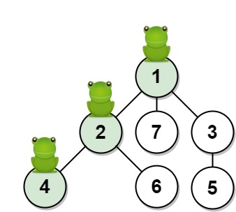
Input: n = 7, edges = [[1,2],[1,3],[1,7],[2,4],[2,6],[3,5]], t = 2, target = 4
Output: 0.16666666666666666
Explanation: The figure above shows the given graph. The frog starts at vertex 1, jumping with 1/3 probability to the vertex 2 after second 1 and then jumping with 1/2 probability to vertex 4 after second 2. Thus the probability for the frog is on the vertex 4 after 2 seconds is 1/3 * 1/2 = 1/6 = 0.16666666666666666.
Example 2:
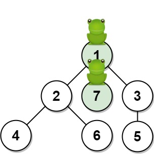
Input: n = 7, edges = [[1,2],[1,3],[1,7],[2,4],[2,6],[3,5]], t = 1, target = 7
Output: 0.3333333333333333
Explanation: The figure above shows the given graph. The frog starts at vertex 1, jumping with 1/3 = 0.3333333333333333 probability to the vertex 7 after second 1.
Constraints:
1 <= n <= 100edges.length == n - 1edges[i].length == 21 <= ai, bi <= n1 <= t <= 501 <= target <= nProblem Overview: You are given an undirected tree with n nodes. A frog starts at node 1 and every second jumps to one of its unvisited neighbors with equal probability. After t seconds, compute the probability that the frog is at the target node. The challenge is modeling the probability flow across the tree while respecting the rule that the frog cannot revisit nodes.
Approach 1: Recursive DFS with Probability Tracking (O(n) time, O(n) space)
This approach treats the tree as a probability flow problem. Build an adjacency list and run a DFS from node 1. At each node, count how many unvisited neighbors are available. If the frog has k choices, each branch receives probability current_prob / k. The recursion continues until either the time reaches t or the frog reaches a leaf. Special handling is required when the frog reaches the target before time runs out: the probability is valid only if the node has no unvisited neighbors left (the frog stays put). DFS works well because it naturally follows paths while carrying probability and time as parameters. The traversal touches each node once, giving O(n) time and O(n) recursion stack space. This approach fits naturally with problems involving trees and probabilistic branching, similar to many Depth-First Search patterns.
Approach 2: BFS with Level Tracking (O(n) time, O(n) space)
A BFS simulation models the frog’s movement second by second. Start with a queue containing (node=1, probability=1.0). Each BFS level represents one second of time. When processing a node, compute how many unvisited neighbors it has and distribute the probability evenly among them before pushing them into the queue. Mark nodes as visited to enforce the rule that the frog never jumps backward. If a node has no unvisited neighbors, its probability remains at that node for the remaining time steps. BFS is often easier to reason about because the queue already aligns with time progression. Each edge is processed at most once, resulting in O(n) time and O(n) queue storage. This technique is common when working with Breadth-First Search on a graph where state evolves per level.
Recommended for interviews: Both DFS and BFS achieve optimal O(n) complexity. Interviewers usually expect the DFS probability propagation because it shows strong reasoning about tree traversal and branching probabilities. BFS is equally valid and sometimes easier to implement without recursion. Showing both approaches demonstrates that you understand tree traversal patterns and how probability flows through a graph structure.
This approach uses Depth First Search (DFS) to simulate the frog's jumps. We track the probability of the frog being on a certain vertex at a particular time. Starting from vertex 1, at each step, we recursively move to all unvisited connected vertices, multiplying the probability by the inverse of the number of possible moves. If the time reaches 't', we check if the current position is the target.
The solution constructs the graph using a dictionary of lists. The recursive function dfs is used to track the probability of the frog reaching the target vertex. It returns the probability of ending at 'target' when time reaches 't'. If we're on a leaf node before time 't', the probability accumulates based on whether the current node is the target or not.
Time Complexity: O(n), as we might need to visit each node once during traversal.
Space Complexity: O(n) for storing the adjacency list of the graph and the recursion stack.
This approach uses Breadth First Search (BFS) to explore the tree level by level. At each level, we update the probability of the frog being on a specific vertex. The exploration stops once either reaching 't' time limit or a vertex with no unvisited children if reached earlier.
The BFS solution iteratively explores each level of the tree, tracking the probability of reaching each vertex. Queue is used to maintain the current node, its probability, and time. This method ensures each vertex is explored uniformly, sharing the probability among children. The BFS loop ends when either the maximum time is reached, or a leaf node is encountered prematurely.
JavaScript
C#
Time Complexity: O(n), due to each edge being processed once.
Space Complexity: O(n), for queue storage handling vertex levels and visited tracking.
First, based on the undirected tree edges given in the problem, we construct an adjacency list g, where g[u] represents all adjacent vertices of vertex u.
Then, we define the following data structures:
q, used to store the vertices and their probabilities for each round of search. Initially, q = [(1, 1.0)], indicating that the probability of the frog being at vertex 1 is 1.0;vis, used to record whether each vertex has been visited. Initially, vis[1] = true, and all other elements are false.Next, we start the breadth-first search.
In each round of search, we take out the head element (u, p) of the queue, where u and p represent the current vertex and its probability, respectively. The number of unvisited adjacent vertices of the current vertex u is denoted as cnt.
u = target, it means that the frog has reached the target vertex. At this time, we judge whether the frog reaches the target vertex in t seconds, or it reaches the target vertex in less than t seconds but cannot jump to other vertices (i.e., t=0 or cnt=0). If so, return p, otherwise return 0.u neq target, we evenly distribute the probability p to all unvisited adjacent vertices of u, then add these vertices to the queue q, and mark these vertices as visited.At the end of a round of search, we decrease t by 1, and then continue the next round of search until the queue is empty or t \lt 0.
| Approach | Complexity |
|---|---|
| Recursive DFS with Probability Tracking | Time Complexity: |
| BFS with Level Tracking | Time Complexity: |
| BFS | — |
| Approach | Time | Space | When to Use |
|---|---|---|---|
| Recursive DFS with Probability Tracking | O(n) | O(n) | When exploring paths with probability propagation in trees |
| BFS with Level Tracking | O(n) | O(n) | When modeling movement step-by-step across time levels |
Leetcode 1377(Hard) Frog Position After T Seconds : Simple C++ Solution • Shivam Patel • 2,505 views views
Watch 9 more video solutions →Practice Frog Position After T Seconds with our built-in code editor and test cases.
Practice on FleetCodePractice this problem
Open in Editor