Watch 10 video solutions for Water Bottles II, a medium level problem involving Math, Simulation. This walkthrough by codestorywithMIK has 4,037 views views. Want to try solving it yourself? Practice on FleetCode or read the detailed text solution.
You are given two integers numBottles and numExchange.
numBottles represents the number of full water bottles that you initially have. In one operation, you can perform one of the following operations:
numExchange empty bottles with one full water bottle. Then, increase numExchange by one.Note that you cannot exchange multiple batches of empty bottles for the same value of numExchange. For example, if numBottles == 3 and numExchange == 1, you cannot exchange 3 empty water bottles for 3 full bottles.
Return the maximum number of water bottles you can drink.
Example 1:
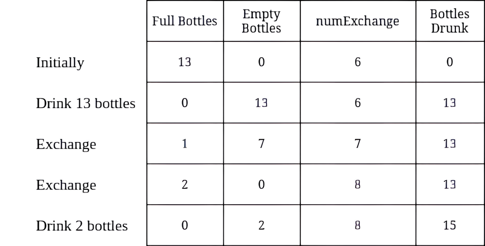
Input: numBottles = 13, numExchange = 6
Output: 15
Explanation: The table above shows the number of full water bottles, empty water bottles, the value of numExchange, and the number of bottles drunk.
Example 2:
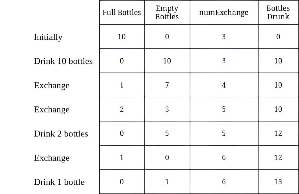
Input: numBottles = 10, numExchange = 3
Output: 13
Explanation: The table above shows the number of full water bottles, empty water bottles, the value of numExchange, and the number of bottles drunk.
Constraints:
1 <= numBottles <= 100 1 <= numExchange <= 100Problem Overview: You start with numBottles full bottles and can exchange empty bottles for a new full one. The catch: after every exchange, the number of empties required increases by 1. The task is to compute the maximum number of bottles you can drink.
Approach 1: Iterative Simulation (Time: O(k), Space: O(1))
This approach directly simulates the process described in the problem. Start by drinking all initial bottles, which gives you the same number of empty bottles. While the number of empty bottles is at least the current exchange requirement (numExchange), perform an exchange: spend the required empties, gain one full bottle, drink it, and increase the exchange cost by one. Each iteration represents a single exchange operation. The logic is simple and mirrors the rules exactly, making it easy to reason about and implement using basic simulation. Time complexity is O(k), where k is the number of exchanges performed, and space complexity is O(1).
The key insight is that every exchange consumes cost empty bottles but returns one new empty after drinking the obtained bottle. The net change in empties per exchange is therefore -(cost - 1). As the required exchange cost keeps increasing, the loop eventually terminates when there are not enough empty bottles left.
Approach 2: Mathematical Optimization (Time: O(1), Space: O(1))
The simulation can be replaced with a mathematical observation. Suppose you perform k exchanges. The exchange costs form an increasing sequence: numExchange, numExchange + 1, ..., numExchange + k - 1. The total number of empty bottles spent is the sum of this arithmetic progression. Each exchange also produces one new empty bottle after drinking the obtained bottle. Using math, the remaining empty bottles after k exchanges can be expressed as:
empties = numBottles - (numExchange + (numExchange+1) + ... + (numExchange+k-1)) + k
This simplifies to numBottles - (k * numExchange + k(k-1)/2) + k. The valid number of exchanges is the largest k such that before each step you still have enough empties to pay the required cost. Solving this inequality allows you to compute k directly using arithmetic progression formulas. The final answer becomes numBottles + k. This approach eliminates iteration entirely and relies on arithmetic reasoning, which is common in problems tagged with Math.
Recommended for interviews: The iterative simulation is usually expected first because it clearly follows the rules of the problem and is easy to verify. It demonstrates solid reasoning and careful state updates. The mathematical optimization is a strong follow‑up that shows deeper insight into arithmetic progressions and constraint analysis. In most interviews, presenting the simulation first and then deriving the constant‑time optimization shows both correctness and problem‑solving depth.
| Approach | Time | Space | When to Use |
|---|---|---|---|
| Iterative Simulation | O(k) | O(1) | Best for clarity and interviews where straightforward simulation of the rules is expected. |
| Mathematical Optimization | O(1) | O(1) | When you recognize the arithmetic progression pattern and want a constant-time calculation. |