Watch 10 video solutions for Spiral Matrix II, a medium level problem involving Array, Matrix, Simulation. This walkthrough by Algorithms Made Easy has 23,965 views views. Want to try solving it yourself? Practice on FleetCode or read the detailed text solution.
Given a positive integer n, generate an n x n matrix filled with elements from 1 to n2 in spiral order.
Example 1:
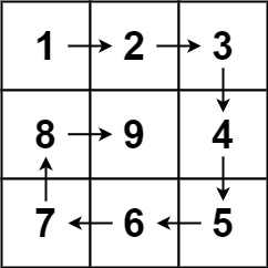
Input: n = 3
Output: [[1,2,3],[8,9,4],[7,6,5]]
Example 2:
Input: n = 1
Output: [[1]]
Constraints:
1 <= n <= 20Problem Overview: Given an integer n, generate an n x n matrix filled with numbers from 1 to n^2 arranged in spiral order. You start at the top-left corner, move right across the first row, then down the last column, left across the bottom row, and continue spiraling inward until the matrix is filled.
Approach 1: Boundary-Based Spiral Simulation (O(n^2) time, O(1) extra space)
This approach simulates the spiral traversal while filling numbers sequentially. Maintain four boundaries: top, bottom, left, and right. Fill the top row from left to right, increment top. Then fill the right column from top to bottom, decrement right. Continue with the bottom row (right to left) and the left column (bottom to top), shrinking the boundaries after each pass. Each iteration writes values directly into the matrix while incrementing the current number.
The key insight is that every spiral "layer" of the matrix can be processed using these four directional passes. By tightening the boundaries after each pass, the algorithm naturally moves inward to the next layer. Every cell is written exactly once, giving O(n^2) time complexity with only constant extra variables.
This is a classic matrix traversal pattern often used in problems involving spiral order traversal or layered processing. The algorithm relies on simple index manipulation within a 2D array and controlled directional movement, making it a clean example of simulation-based problem solving.
Approach 2: Direction Vector Simulation (O(n^2) time, O(1) extra space)
Another implementation tracks the current direction using vectors such as (0,1), (1,0), (0,-1), and (-1,0) for right, down, left, and up. Start at position (0,0) and place numbers sequentially. Before each step, check whether the next cell would go out of bounds or hit a previously filled cell. If so, rotate to the next direction in the cycle.
This version models the spiral movement explicitly and avoids maintaining four boundaries. The logic is slightly more dynamic but still fills exactly n^2 cells with constant extra memory. Many engineers prefer the boundary method for clarity, while the direction-vector method is useful when implementing generalized grid traversal patterns.
Recommended for interviews: The boundary-based spiral simulation is the expected solution. It shows you understand layered matrix traversal and can control indices carefully. The direction-vector version also works, but interviewers typically prefer the boundary approach because it is easier to reason about and implement without edge-case mistakes.
| Approach | Time | Space | When to Use |
|---|---|---|---|
| Boundary-Based Spiral Simulation | O(n^2) | O(1) | Best general solution for generating spiral matrices; simple logic with clear boundary updates |
| Direction Vector Simulation | O(n^2) | O(1) | Useful when implementing generalized grid movement or when direction-based traversal is preferred |