Given an m x n matrix, return all elements of the matrix in spiral order.
Example 1:
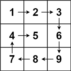
Input: matrix = [[1,2,3],[4,5,6],[7,8,9]]
Output: [1,2,3,6,9,8,7,4,5]
Example 2:

Input: matrix = [[1,2,3,4],[5,6,7,8],[9,10,11,12]]
Output: [1,2,3,4,8,12,11,10,9,5,6,7]
Constraints:
m == matrix.lengthn == matrix[i].length1 <= m, n <= 10-100 <= matrix[i][j] <= 100Problem Overview: Given an m × n matrix, return all elements in spiral order. The traversal starts at the top-left corner, moves right across the first row, then down the last column, then left across the bottom row, and continues inward layer by layer until every element is visited.
Approach 1: Iterative Boundary Management (O(m×n) time, O(1) space)
This approach simulates the spiral traversal by maintaining four boundaries: top, bottom, left, and right. You iterate across the top row, then move down the right column, then traverse the bottom row in reverse, and finally move up the left column. After completing each direction, adjust the corresponding boundary inward. The key insight is that every spiral layer shrinks the valid traversal region. Each matrix element is visited exactly once, giving O(m×n) time with constant extra space. This method fits naturally with problems involving array traversal and matrix boundary processing.
Approach 2: Recursive Divide and Conquer (O(m×n) time, O(m+n) recursion space)
The matrix can also be processed layer by layer using recursion. Each recursive call handles one outer ring of the matrix: traverse the top row, right column, bottom row (reverse), and left column (reverse). After processing the outer layer, the recursion continues with the inner submatrix defined by updated boundaries. The recursive structure mirrors the spiral pattern directly, which can make the logic easier to reason about. The tradeoff is additional recursion stack usage proportional to the number of layers, typically O(min(m,n)). This approach is a natural fit when practicing simulation or divide-and-conquer thinking.
Recommended for interviews: Iterative boundary management is the expected solution. Interviewers want to see careful boundary updates and correct handling of edge cases when rows or columns collapse. The recursive version demonstrates conceptual clarity but rarely improves performance. Showing the iterative solution proves you can control indices precisely and implement efficient matrix traversal.
This approach involves simulating the spiral order by iteratively traversing matrix layers. The boundaries are adjusted after each complete traversal of a side (top, right, bottom, left). By shrinking the boundaries, we can eventually cover the entire matrix in a spiral order.
The C solution uses a while loop to traverse the matrix. It defines boundaries for the layers (top, bottom, left, right) and adjusts these boundaries after completing the traversal of each side. The movement is controlled by the boundary variables, ensuring the entire matrix is spirally covered.
Time Complexity: O(m * n) where m is the number of rows and n is the number of columns, since each element is accessed once.
Space Complexity: O(1) additional space, excluding the space for the output array.
This approach uses recursion to divide the matrix into smaller sections. By processing the outer layer of the matrix, we can recursively call the function on the remaining submatrix. This continues until the entire matrix is covered.
The Python solution defines a recursive helper function `spiral_layer`, with parameters defining the boundaries of the current submatrix. The base condition checks if the boundary indices are valid. It extracts and appends elements to the result, then recursively narrows the boundaries until they converge.
Python
Time Complexity: O(m * n) since each recursive call processes an entire layer of the matrix.
Space Complexity: O(m * n) due to the recursive call stack usage, although tail recursion may optimize this depending on the Python implementation.
We can simulate the entire traversal process. We use i and j to represent the row and column of the current element being visited, and k to represent the current direction. We use an array or hash table vis to record whether each element has been visited. Each time we visit an element, we mark it as visited, then move one step forward in the current direction. If moving forward results in an out-of-bounds condition or the element has already been visited, we change direction and continue moving forward until the entire matrix has been traversed.
The time complexity is O(m times n), and the space complexity is O(m times n). Here, m and n are the number of rows and columns of the matrix, respectively.
Python
Java
C++
Go
TypeScript
Rust
JavaScript
C#
Notice that the range of matrix element values is [-100, 100]. Therefore, we can add a large value, such as 300, to the visited elements. This way, we only need to check if the visited element is greater than 100, without needing extra space to record whether it has been visited. If we need to restore the original values of the visited elements, we can traverse the matrix again after the traversal is complete and subtract 300 from all elements.
The time complexity is O(m times n), where m and n are the number of rows and columns of the matrix, respectively. The space complexity is O(1).
Python
Java
C++
Go
TypeScript
Rust
JavaScript
C#
| Approach | Complexity |
|---|---|
| Iterative Boundary Management | Time Complexity: O(m * n) where m is the number of rows and n is the number of columns, since each element is accessed once. Space Complexity: O(1) additional space, excluding the space for the output array. |
| Recursive Divide and Conquer | Time Complexity: O(m * n) since each recursive call processes an entire layer of the matrix. Space Complexity: O(m * n) due to the recursive call stack usage, although tail recursion may optimize this depending on the Python implementation. |
| Simulation | — |
| Simulation (Space Optimization) | — |
| Approach | Time | Space | When to Use |
|---|---|---|---|
| Iterative Boundary Management | O(m×n) | O(1) | Best general solution. Efficient traversal with constant extra memory. |
| Recursive Divide and Conquer | O(m×n) | O(m+n) recursion stack | Useful for conceptual clarity or recursion practice when processing matrix layers. |
Spiral Matrix - Microsoft Interview Question - Leetcode 54 • NeetCode • 231,899 views views
Watch 9 more video solutions →Practice Spiral Matrix with our built-in code editor and test cases.
Practice on FleetCodePractice this problem
Open in Editor