Given a 2D grid of size m x n and an integer k. You need to shift the grid k times.
In one shift operation:
grid[i][j] moves to grid[i][j + 1].grid[i][n - 1] moves to grid[i + 1][0].grid[m - 1][n - 1] moves to grid[0][0].Return the 2D grid after applying shift operation k times.
Example 1:
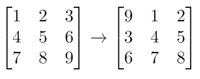
Input: grid = [[1,2,3],[4,5,6],[7,8,9]], k = 1
Output: [[9,1,2],[3,4,5],[6,7,8]]
Example 2:
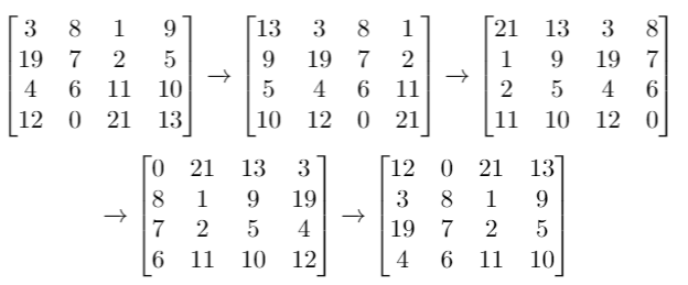
Input: grid = [[3,8,1,9],[19,7,2,5],[4,6,11,10],[12,0,21,13]], k = 4
Output: [[12,0,21,13],[3,8,1,9],[19,7,2,5],[4,6,11,10]]
Example 3:
Input: grid = [[1,2,3],[4,5,6],[7,8,9]], k = 9
Output: [[1,2,3],[4,5,6],[7,8,9]]
Constraints:
m == grid.lengthn == grid[i].length1 <= m <= 501 <= n <= 50-1000 <= grid[i][j] <= 10000 <= k <= 100Problem Overview: You receive an m x n grid and an integer k. Each shift moves every element one step to the right, the last element of a row becomes the first of the next row, and the bottom‑right element wraps to the top‑left. After performing the shift operation k times, return the final grid configuration.
Approach 1: 1D Array Transformation (Time: O(mn), Space: O(mn))
The key observation is that the grid behaves like a single circular array of length m * n. Flatten the array/matrix indices into a 1D index using index = row * n + col. After k shifts, the element moves to (index + k) % (m * n). Convert that new index back to 2D coordinates using division and modulo.
This avoids performing the shift operation repeatedly. Instead, iterate through the grid once, compute the destination index, and place the element in the result grid. The approach is clean and deterministic: one pass to map positions and rebuild the grid. Time complexity stays O(mn) regardless of k, and space complexity is O(mn) for the new grid.
Approach 2: In-Place Simulation (Time: O(kmn), Space: O(1))
This method directly simulates the shift operation exactly as described. For each shift, traverse the grid from the bottom‑right corner while carrying the previous value that should move into the current cell. The value from the last cell wraps around to the first position.
Although you can reduce unnecessary work by computing k = k % (m * n), each shift still requires scanning the entire matrix. That results in O(kmn) time in the worst case. The advantage is constant extra memory because the transformation happens directly inside the grid. This technique mirrors the problem’s simulation behavior and is easy to reason about step by step.
Recommended for interviews: The 1D index transformation is the expected solution. It shows you recognize that a 2D grid can be treated as a circular linear structure and optimized using modular arithmetic. Interviewers often accept the simulation approach first because it demonstrates understanding of the shift rules, but the index‑mapping solution proves stronger algorithmic thinking with optimal O(mn) time.
Transform the 2D grid into a 1D list: The problem of shifting all elements in a 2D grid can be simplified by flattening the grid into a 1D array. This enables easier shifting and indexing.
Shift the 1D Array: Determine the actual number of shifts needed by computing k % (m * n) to avoid redundant full rotations. Then partition and concatenate the 1D array accordingly to achieve the desired shift.
Transform back to 2D Grid: Finally, map the shifted 1D list back to the original 2D grid layout.
This C solution first calculates the equivalent shift for the 1D representation of the grid. The nested loop traverses each element in the current 2D grid and calculates its new position in the shifted grid using the offset calculated with the modulo operation.
Time Complexity: O(m * n) since we access each grid element once.
Space Complexity: O(m * n) needed for the result grid storage.
Calculate Direct Position Mapping: Instead of flattening, calculate the direct position mapping for shifted elements. This avoids the extra space used by intermediate lists.
Perform Element-wise Placement: Iterate through elements and directly place them in their new calculated positions.
The C version for direct mapping ensures each element’s target location is computed directly, with careful attention to index wrap-around using modulus.
Time Complexity: O(m * n).
Space Complexity: O(m * n) for the shifted result.
According to the problem description, if we flatten the 2D array into a 1D array, then each shift operation is to move the elements in the array one position to the right, with the last element moving to the first position of the array.
Therefore, we can flatten the 2D array into a 1D array, then calculate the final position idx = (x, y) of each element, and update the answer array ans[x][y] = grid[i][j].
The time complexity is O(m times n), where m and n are the number of rows and columns in the grid array, respectively. We need to traverse the grid array once to calculate the final position of each element. Ignoring the space consumption of the answer array, the space complexity is O(1).
Python
Java
C++
Go
TypeScript
| Approach | Complexity |
|---|---|
| Approach 1: 1D Array Transformation | Time Complexity: O(m * n) since we access each grid element once. |
| Approach 2: In-Place Simulation | Time Complexity: O(m * n). |
| Flattening the 2D Array | — |
| Approach | Time | Space | When to Use |
|---|---|---|---|
| 1D Array Transformation | O(mn) | O(mn) | Best general solution. Converts the grid to a circular 1D index and computes final positions directly. |
| In-Place Simulation | O(kmn) | O(1) | Useful when minimizing extra memory or when demonstrating the shift mechanics step by step. |
Shift 2D Grid - Leetcode 1260 - Python • NeetCode • 23,342 views views
Watch 9 more video solutions →Practice Shift 2D Grid with our built-in code editor and test cases.
Practice on FleetCode