Given the root of a binary tree, construct a 0-indexed m x n string matrix res that represents a formatted layout of the tree. The formatted layout matrix should be constructed using the following rules:
height and the number of rows m should be equal to height + 1.n should be equal to 2height+1 - 1.res[0][(n-1)/2]).res[r][c], place its left child at res[r+1][c-2height-r-1] and its right child at res[r+1][c+2height-r-1]."".Return the constructed matrix res.
Example 1:
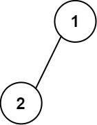
Input: root = [1,2]
Output:
[["","1",""],
 ["2","",""]]
Example 2:
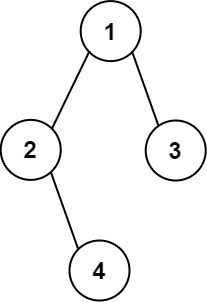
Input: root = [1,2,3,null,4]
Output:
[["","","","1","","",""],
 ["","2","","","","3",""],
 ["","","4","","","",""]]
Constraints:
[1, 210].-99 <= Node.val <= 99[1, 10].Problem Overview: Given the root of a binary tree, return a 2D string matrix that visually represents the tree structure. The matrix width must be 2^height - 1, and each node is placed at the midpoint of its valid column range so that left and right children appear symmetrically below the parent.
Approach 1: Recursive Placement of Nodes (DFS) (Time: O(n), Space: O(n))
This approach uses Depth-First Search to place nodes directly in the correct matrix positions. First compute the tree height using a recursive traversal. The matrix dimensions become height x (2^height - 1). During DFS, each node is assigned a column based on the midpoint of its current column range [left, right]. Place the node value at that midpoint, then recursively process the left child with range [left, mid-1] and the right child with [mid+1, right]. This works because every subtree occupies exactly half of its parent’s horizontal space. The recursion naturally mirrors the structure of a Binary Tree, making the placement logic clean and predictable. This is the most common and readable solution.
Approach 2: Iterative Level Order Traversal (BFS) (Time: O(n), Space: O(n))
This version uses Breadth-First Search with a queue to process nodes level by level. After computing the tree height and initializing the matrix, push the root into a queue along with its column boundaries. Each queue entry stores (node, row, leftBound, rightBound). When processing a node, compute the midpoint column and write its value into the matrix. Then push the left and right children into the queue with updated column ranges. BFS makes the row index explicit and avoids recursion depth limits. The placement logic is the same midpoint calculation used in the DFS solution, but controlled iteratively.
Recommended for interviews: The recursive DFS placement is usually the expected solution because it maps directly to the tree structure and requires less bookkeeping. Interviewers like it because the midpoint calculation clearly shows you understand how the visual layout relates to tree height. The BFS approach is equally optimal in complexity and demonstrates familiarity with queue-based traversal, but the DFS version is typically shorter and easier to reason about.
This approach involves calculating the height of the binary tree first. Once we have the height, we can determine the size of the resulting matrix with m = height + 1 and n = 2height + 1 - 1. We then recursively place each node starting from the root at res[0][(n-1)/2]. For any node at position res[r][c], its left child is placed at res[r+1][c-2height-r-1] and its right child at res[r+1][c+2height-r-1].
First, we calculate the height of the tree to determine the dimensions of the result matrix. Then, using recursion, we place each node at its appropriate position. The recursive function fill places the root at the center and calculates positions for child nodes using a power of two shifts according to their level in the tree.
Time Complexity: O(m * n), where m and n are the dimensions of the matrix. The recursive function visits each node once.
Space Complexity: O(m * n) for the result matrix.
This approach uses an iterative method, leveraging a queue for level order traversal to place nodes in the matrix. We still need to calculate the height first to know the matrix size. Using a queue, nodes are enqueued with their respective positions, and at each level, node positions are calculated based on their level and placed in the matrix iteratively.
This solution utilizes an iterative approach with a queue for BFS-like level order traversal. In this method, all nodes are processed level by level, and their positions are calculated without recursion by using a queue to manage each node and its column index.
Time Complexity: O(m * n), as we traverse the tree and fill the matrix.
Space Complexity: O(m * n) for storing the output matrix.
| Approach | Complexity |
|---|---|
| Recursive Placement of Nodes | Time Complexity: |
| Iterative Level Order Traversal | Time Complexity: |
| Default Approach | — |
| Approach | Time | Space | When to Use |
|---|---|---|---|
| Recursive Placement of Nodes (DFS) | O(n) | O(n) | Best general solution. Clean recursion that mirrors the tree structure. |
| Iterative Level Order Traversal (BFS) | O(n) | O(n) | Useful when avoiding recursion or when explicitly processing nodes by level. |
花花酱 LeetCode 655. Print Binary Tree - 刷题找工作 EP9 • Hua Hua • 5,735 views views
Watch 6 more video solutions →Practice Print Binary Tree with our built-in code editor and test cases.
Practice on FleetCode