
Number of Good Leaf Nodes Pairs - Solution & Explanation
Problem Statement
You are given the root of a binary tree and an integer distance. A pair of two different leaf nodes of a binary tree is said to be good if the length of the shortest path between them is less than or equal to distance.
Return the number of good leaf node pairs in the tree.
Example 1:
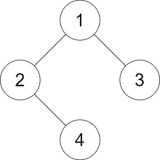
Input: root = [1,2,3,null,4], distance = 3
Output: 1
Explanation: The leaf nodes of the tree are 3 and 4 and the length of the shortest path between them is 3. This is the only good pair.
Example 2:
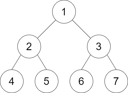
Input: root = [1,2,3,4,5,6,7], distance = 3
Output: 2
Explanation: The good pairs are [4,5] and [6,7] with shortest path = 2. The pair [4,6] is not good because the length of ther shortest path between them is 4.
Example 3:
Input: root = [7,1,4,6,null,5,3,null,null,null,null,null,2], distance = 3
Output: 1
Explanation: The only good pair is [2,5].
Constraints:
- The number of nodes in the
treeis in the range[1, 210]. 1 <= Node.val <= 1001 <= distance <= 10
Approach Overview
Problem Overview: Given a binary tree and an integer distance, count pairs of leaf nodes whose shortest path length is less than or equal to that distance. The path length is measured by the number of edges between the two leaves.
Approach 1: DFS with Distance Array (O(n · d²) time, O(h · d) space)
Use a postorder depth-first search to aggregate distances from leaf nodes upward. Each recursive call returns an array where index i represents how many leaf nodes exist at distance i from the current node. For leaf nodes, return an array with distance 1. When processing an internal node, combine the left and right arrays: iterate through all pairs of distances i and j and count pairs where i + j ≤ distance. Then build a new array for the parent by shifting distances by one edge. The key insight is that every valid pair must have its lowest common ancestor at some node visited during DFS, so counting during the merge step captures all valid pairs efficiently.
This approach keeps the distance arrays capped at the maximum allowed distance, which keeps the merge step small. Since distance ≤ 10 in constraints, the nested loop over distances is effectively constant. The algorithm visits each node once and performs small merges, giving near-linear performance for practical inputs.
Approach 2: Preprocessing with Dynamic Programming (O(n · d²) time, O(n · d) space)
Another strategy treats each node as a subproblem and stores the number of leaves at each distance within its subtree. Using tree-based dynamic programming, compute a DP table where dp[node][k] represents how many leaf nodes exist at distance k from that node. Build this table bottom-up during a traversal of the tree. When combining children, compute cross-subtree leaf pairs by checking all i from the left subtree and j from the right subtree where i + j ≤ distance. Then shift distances by one to populate the current node's DP row.
This method makes the state explicit and can be easier to reason about if you think in terms of subtree summaries. The tradeoff is higher memory usage since each node keeps its own distance table instead of returning temporary arrays.
Recommended for interviews: DFS with distance arrays. It demonstrates strong understanding of tree traversal, subtree aggregation, and lowest common ancestor reasoning. Interviewers expect candidates to recognize that valid leaf pairs must meet at an internal node and can be counted during a postorder merge. Explaining the brute force idea (checking all leaf pairs with LCA or BFS) shows baseline understanding, but the DFS aggregation approach shows stronger algorithmic design.
Approach 1: DFS with Distance Array
This approach involves a DFS traversal of the tree. For each node, we compute the number of leaf nodes at each possible distance. We merge the results from the left and right subtrees and count the valid leaf pairs.
In this C implementation of the DFS approach, we maintain arrays to count leaf nodes at particular distances for each subtree. We combine these left and right arrays for each node and calculate valid pairs within the distance constraint. The result is accumulated during the traversal.
Complexity
Time Complexity: O(n * distance) due to traversing the entire tree and computing leaf pairs.
Space Complexity: O(distance) for storing distance arrays.
Approach 2: Preprocessing with Dynamic Programming
This approach leverages preprocessing leaf distances in a dynamic programming table, which gives quick lookups during pair evaluation. It builds the DP table during a DFS traversal, allowing efficient pair computation afterward.
A solution in C would involve more detailed memory management and array calculations for storing and evaluating distances.
Complexity
Time Complexity: Approximately O(n^2) for thorough pairing and evaluation.
Space Complexity: O(n^2) due to pair-wise distance visualization.
Approach 3: Recursion
The problem asks for the number of good leaf node pairs in a binary tree. The answer can be divided into three parts: the number of good leaf node pairs in the left subtree, the number of good leaf node pairs in the right subtree, and the number of good leaf node pairs formed by leaf nodes from the left subtree and leaf nodes from the right subtree.
We can solve this recursively.
The time complexity is O(n times d^2 times h), where n is the number of nodes in the binary tree, and h and d are the height of the binary tree and the distance limit, respectively. The space complexity is O(h) for the recursion stack.
Code
Python
Java
C++
Go
TypeScript
JavaScript
Complexity Comparison
| Approach | Complexity |
|---|---|
| DFS with Distance Array | Time Complexity: O(n * distance) due to traversing the entire tree and computing leaf pairs. |
| Preprocessing with Dynamic Programming | Time Complexity: Approximately O(n^2) for thorough pairing and evaluation. |
| Recursion | — |
Detailed Complexity Analysis
| Approach | Time | Space | When to Use |
|---|---|---|---|
| DFS with Distance Array | O(n · d²) | O(h · d) | Best general solution for interviews and coding platforms; efficient when the distance limit is small. |
| Preprocessing with Dynamic Programming | O(n · d²) | O(n · d) | Useful when you want explicit subtree DP states or need reusable distance data for additional queries. |
Video Solution
Number of Good Leaf Nodes Pairs - Leetcode 1530 - Python • NeetCodeIO • 14,015 views views
Watch 9 more video solutions →Frequently Asked Questions
Is Number of Good Leaf Nodes Pairs easy or hard?
Number of Good Leaf Nodes Pairs Python/Java solution
How to solve Number of Good Leaf Nodes Pairs in O(n)?
What is the best approach for Number of Good Leaf Nodes Pairs?
Is Number of Good Leaf Nodes Pairs asked at Google/Amazon/Meta?
What data structure is used in Number of Good Leaf Nodes Pairs?
What is the time complexity of Number of Good Leaf Nodes Pairs?
Ready to solve this problem?
Practice Number of Good Leaf Nodes Pairs with our built-in code editor and test cases.
Practice on FleetCode