There exist two undirected trees with n and m nodes, labeled from [0, n - 1] and [0, m - 1], respectively.
You are given two 2D integer arrays edges1 and edges2 of lengths n - 1 and m - 1, respectively, where edges1[i] = [ai, bi] indicates that there is an edge between nodes ai and bi in the first tree and edges2[i] = [ui, vi] indicates that there is an edge between nodes ui and vi in the second tree.
Node u is target to node v if the number of edges on the path from u to v is even. Note that a node is always target to itself.
Return an array of n integers answer, where answer[i] is the maximum possible number of nodes that are target to node i of the first tree if you had to connect one node from the first tree to another node in the second tree.
Note that queries are independent from each other. That is, for every query you will remove the added edge before proceeding to the next query.
Example 1:
Input: edges1 = [[0,1],[0,2],[2,3],[2,4]], edges2 = [[0,1],[0,2],[0,3],[2,7],[1,4],[4,5],[4,6]]
Output: [8,7,7,8,8]
Explanation:
i = 0, connect node 0 from the first tree to node 0 from the second tree.i = 1, connect node 1 from the first tree to node 4 from the second tree.i = 2, connect node 2 from the first tree to node 7 from the second tree.i = 3, connect node 3 from the first tree to node 0 from the second tree.i = 4, connect node 4 from the first tree to node 4 from the second tree.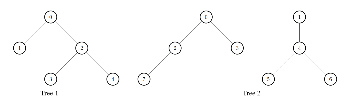
Example 2:
Input: edges1 = [[0,1],[0,2],[0,3],[0,4]], edges2 = [[0,1],[1,2],[2,3]]
Output: [3,6,6,6,6]
Explanation:
For every i, connect node i of the first tree with any node of the second tree.

Constraints:
2 <= n, m <= 105edges1.length == n - 1edges2.length == m - 1edges1[i].length == edges2[i].length == 2edges1[i] = [ai, bi]0 <= ai, bi < nedges2[i] = [ui, vi]0 <= ui, vi < medges1 and edges2 represent valid trees.Problem Overview: You are given two trees. You may connect one node from the first tree to any node in the second tree. After adding this edge, determine for every node in the first tree the maximum number of target nodes reachable at even distance. The challenge is choosing the best connection point in the second tree while efficiently computing parity distances.
Approach 1: DFS with Pre-computed Parities (O(n + m) time, O(n + m) space)
Trees are bipartite by nature. If you run a depth-first search on each tree, you can assign every node a parity (0 for even depth, 1 for odd depth). Count how many nodes belong to each parity group. For the first tree, each node already knows how many nodes are at even distance within its own tree based on its parity group. For the second tree, you only need the larger of the two parity groups because you can connect the trees in a way that flips parity if beneficial. Iterate through nodes in tree1 and combine its reachable even-parity count with the best possible count from tree2. This avoids recomputing distances for every possible connection.
The key insight: adding a single edge toggles parity depending on which nodes you connect. Because parity is all that matters for even-distance checks, precomputing counts for both parity sets gives the optimal answer immediately.
Approach 2: Dynamic Programming with Path Parity Tracking (O(n + m) time, O(n + m) space)
Another approach tracks parity contributions using reroot-style tree dynamic programming. Run a traversal on each tree and compute how many nodes are reachable with even and odd parity from every node. While traversing, propagate counts to children while flipping parity as edges are crossed. This technique resembles rerooting DP frequently used in tree problems. After computing parity distributions, evaluate the best connection between the two trees by combining compatible parity groups. Although the complexity matches the DFS approach, the implementation is more involved because state transitions must correctly adjust parity counts.
Traversal can be implemented with either DFS or BFS. Both produce the same parity labeling since the graph is a tree.
Recommended for interviews: The DFS parity counting approach. It demonstrates recognition of the bipartite property of trees and reduces the problem to simple counting instead of repeated path calculations. Mentioning the brute-force idea (checking every connection with repeated traversals) shows understanding, but the parity observation is the optimization interviewers expect.
To determine the maximum number of nodes in the second tree that are 'target' to a specific node in the first tree, explore the parity of paths in each tree independently using Depth First Search (DFS). For each source node in the first tree, connect it with each node in the second tree to compute the union of target nodes. This requires understanding how the parity of the path from the source node to another node affects its 'target' status.
This solution involves setting up a DFS method to compute path parities in both trees independently. A main routine calls DFS from each node in the first tree, temporarily adds and evaluates connections to nodes in the second tree, allowing us to compare results for each base node efficiently.
Time Complexity: O(n * m) due to checking each second tree node for each first tree node.
Space Complexity: O(n + m) for storing parity and connectivity information in auxiliary arrays.
Alternatively, use dynamic programming to track path parities across disjoint subproblems. Here, linked lists or adjacency tables establish node connections. By leveraging dynamic techniques, each node's potential 'target' connections are recursively built and stored, facilitating rapid evaluations.
This solution focuses on memoizing parity-based results for individual queries. By storing intermediate connectivity results, expensive recalculations are avoided.
Time Complexity: O(n * m) but with reduced recalculation overhead.
Space Complexity: O(n + m) due to memoization arrays and list structures.
The number of target nodes for node i can be divided into two parts:
i.First, we use Depth-First Search (DFS) to calculate the number of nodes in the second tree with the same depth parity, denoted as cnt2. Then, we calculate the number of nodes in the first tree with the same depth parity as node i, denoted as cnt1. Therefore, the number of target nodes for node i is max(cnt2) + cnt1.
The time complexity is O(n + m), and the space complexity is O(n + m). Here, n and m are the number of nodes in the first and second trees, respectively.
| Approach | Complexity |
|---|---|
| DFS with Pre-computed Parities | Time Complexity: O(n * m) due to checking each second tree node for each first tree node. |
| Dynamic Programming with Path Parity Tracking | Time Complexity: O(n * m) but with reduced recalculation overhead. |
| DFS | — |
| Approach | Time | Space | When to Use |
|---|---|---|---|
| Brute Force Recompute Distances | O(n * (n + m)) | O(n + m) | Conceptual baseline; try every possible connection and run BFS/DFS each time |
| DFS with Pre-computed Parities | O(n + m) | O(n + m) | Best practical solution; uses bipartite parity property of trees |
| Dynamic Programming with Path Parity Tracking | O(n + m) | O(n + m) | Useful when extending to rerooting or multi-query tree problems |
Maximize the Number of Target Nodes After Connecting Trees II | Full Dry Run | Leetcode 3373 | MIK • codestorywithMIK • 6,330 views views
Watch 9 more video solutions →Practice Maximize the Number of Target Nodes After Connecting Trees II with our built-in code editor and test cases.
Practice on FleetCodePractice this problem
Open in Editor