You are given an undirected weighted graph of n nodes numbered from 0 to n - 1. The graph consists of m edges represented by a 2D array edges, where edges[i] = [ai, bi, wi] indicates that there is an edge between nodes ai and bi with weight wi.
Consider all the shortest paths from node 0 to node n - 1 in the graph. You need to find a boolean array answer where answer[i] is true if the edge edges[i] is part of at least one shortest path. Otherwise, answer[i] is false.
Return the array answer.
Note that the graph may not be connected.
Example 1:
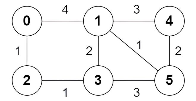
Input: n = 6, edges = [[0,1,4],[0,2,1],[1,3,2],[1,4,3],[1,5,1],[2,3,1],[3,5,3],[4,5,2]]
Output: [true,true,true,false,true,true,true,false]
Explanation:
The following are all the shortest paths between nodes 0 and 5:
0 -> 1 -> 5: The sum of weights is 4 + 1 = 5.0 -> 2 -> 3 -> 5: The sum of weights is 1 + 1 + 3 = 5.0 -> 2 -> 3 -> 1 -> 5: The sum of weights is 1 + 1 + 2 + 1 = 5.Example 2:
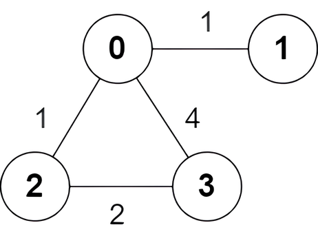
Input: n = 4, edges = [[2,0,1],[0,1,1],[0,3,4],[3,2,2]]
Output: [true,false,false,true]
Explanation:
There is one shortest path between nodes 0 and 3, which is the path 0 -> 2 -> 3 with the sum of weights 1 + 2 = 3.
Constraints:
2 <= n <= 5 * 104m == edges.length1 <= m <= min(5 * 104, n * (n - 1) / 2)0 <= ai, bi < nai != bi1 <= wi <= 105Problem Overview: You are given a weighted graph and must determine which edges appear in at least one shortest path from node 0 to node n-1. Instead of returning the path itself, the goal is to mark every edge that can participate in any optimal route.
Approach 1: Double Dijkstra's Algorithm (O(E log V) time, O(V + E) space)
This approach runs Dijkstra twice. First compute the shortest distance from the source node 0 to every node. Then run Dijkstra again from the target node n-1 (conceptually on the reversed graph, though for undirected graphs the same adjacency list works). Let distStart[u] be the distance from the start and distEnd[v] be the distance from the end. For an edge (u, v, w), the edge belongs to some shortest path if distStart[u] + w + distEnd[v] == distStart[n-1] or the symmetric direction distStart[v] + w + distEnd[u] == distStart[n-1]. The key insight: any shortest path can be decomposed into prefix distance from the start, the edge weight, and suffix distance to the target. If their sum equals the global shortest distance, the edge lies on an optimal path. The heavy lifting is done by a min-heap implementation of priority queue inside Dijkstra. This method works efficiently on large sparse graphs.
Approach 2: Bellman-Ford with Inverse Relaxation (O(V * E) time, O(V + E) space)
This version starts by computing shortest distances from the source using the Bellman-Ford relaxation process. After the distances stabilize, examine each edge to see whether it preserves shortest-path consistency: an edge (u, v, w) is valid if dist[u] + w == dist[v] or dist[v] + w == dist[u]. These edges form a directed acyclic structure that represents all valid shortest-path transitions. Build this filtered graph and run a DFS or BFS from node 0 to find which edges can actually reach n-1. Only edges reachable in this constrained graph belong to some shortest path. Bellman-Ford avoids priority queues and works even if negative weights exist (as long as there are no negative cycles). It relies on repeated relaxation over the full edge list, a classic technique in shortest path problems.
Recommended for interviews: Double Dijkstra is the expected solution. It runs in O(E log V), scales well for dense inputs, and clearly demonstrates understanding of graph shortest path decomposition. Bellman-Ford is a good fallback if negative weights appear or if the interviewer explicitly asks for a relaxation-based approach.
This approach uses Dijkstra's algorithm twice. First, compute the shortest paths from the start node (0) to all other nodes. Then compute the shortest paths from the target node (n-1) to all other nodes by reversing the graph edges. Use these two results to determine if an edge can be part of any shortest path.
This function constructs the graph and uses Dijkstra's algorithm twice to gather the shortest path weights from the start to all nodes and from the end to all nodes (by reversing the graph). It checks if for each edge (u, v), the sum of the shortest path from the start to u, the weight w of the edge, and the shortest path from v to the end equals the shortest path from start to end. If so, the edge is part of at least one shortest path.
Python
C++
Java
JavaScript
Time Complexity: O((n + m) log n), as Dijkstra's algorithm, is run twice, and each involving operations on vertices and edges.
Space Complexity: O(n + m), for storing the graphs and distance arrays.
This approach employs the Bellman-Ford algorithm to find the shortest paths. After determining the shortest paths from the start, we use another Bellman-Ford process but in reverse, allowing edge relaxation from the end node. This method checks if an edge contributes as a segment to any shortest paths.
The Bellman-Ford algorithm is applied twice: once for the original edges to determine distances from the starting node, and once on reversed edges for distances to the end node. It checks edge validity in shortest paths through summation of these measurements compared to the overall shortest path distance.
Python
C++
Java
JavaScript
Time Complexity: O(n * m), as Bellman-Ford is applied twice with edge relaxation.
Space Complexity: O(n), maintaining distance arrays primarily.
First, we create an adjacency list g to store the edges of the graph. Then we create an array dist to store the shortest distance from node 0 to other nodes. We initialize dist[0] = 0, and the distance of other nodes is initialized to infinity.
Then, we use the Dijkstra algorithm to calculate the shortest distance from node 0 to other nodes. The specific steps are as follows:
q to store the distance and node number of the nodes. Initially, add node 0 to the queue with a distance of 0.a from the queue. If the distance da of a is greater than dist[a], it means that a has been updated, so skip it directly.b of node a. If dist[b] > dist[a] + w, update dist[b] = dist[a] + w, and add node b to the queue.Next, we create an answer array ans of length m, initially all elements are false. If dist[n - 1] is infinity, it means that node 0 cannot reach node n - 1, return ans directly. Otherwise, we start from node n - 1, traverse all edges, if the edge (a, b, i) satisfies dist[a] = dist[b] + w, set ans[i] to true, and add node b to the queue.
Finally, return the answer.
The time complexity is O(m times log m), and the space complexity is O(n + m), where n and m are the number of nodes and edges respectively.
| Approach | Complexity |
|---|---|
| Approach 1: Double Dijkstra's Algorithm | Time Complexity: O((n + m) log n), as Dijkstra's algorithm, is run twice, and each involving operations on vertices and edges. Space Complexity: O(n + m), for storing the graphs and distance arrays. |
| Approach 2: Bellman-Ford Algorithm with Inverse Relaxation | Time Complexity: O(n * m), as Bellman-Ford is applied twice with edge relaxation. Space Complexity: O(n), maintaining distance arrays primarily. |
| Heap Optimized Dijkstra | — |
| Approach | Time | Space | When to Use |
|---|---|---|---|
| Double Dijkstra's Algorithm | O(E log V) | O(V + E) | Best general solution for weighted graphs with non-negative edges |
| Bellman-Ford with Inverse Relaxation | O(V * E) | O(V + E) | Useful when negative edge weights are possible or when demonstrating relaxation-based shortest paths |
Find Edges in Shortest Paths | Dijkstra's Algo | Full Intuition | Leetcode 3123 | codestorywithMIK • codestorywithMIK • 5,668 views views
Watch 9 more video solutions →Practice Find Edges in Shortest Paths with our built-in code editor and test cases.
Practice on FleetCodePractice this problem
Open in Editor