There exists an undirected and initially unrooted tree with n nodes indexed from 0 to n - 1. You are given the integer n and a 2D integer array edges of length n - 1, where edges[i] = [ai, bi] indicates that there is an edge between nodes ai and bi in the tree.
Each node has an associated price. You are given an integer array price, where price[i] is the price of the ith node.
The price sum of a given path is the sum of the prices of all nodes lying on that path.
The tree can be rooted at any node root of your choice. The incurred cost after choosing root is the difference between the maximum and minimum price sum amongst all paths starting at root.
Return the maximum possible cost amongst all possible root choices.
Example 1:
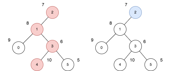
Input: n = 6, edges = [[0,1],[1,2],[1,3],[3,4],[3,5]], price = [9,8,7,6,10,5]
Output: 24
Explanation: The diagram above denotes the tree after rooting it at node 2. The first part (colored in red) shows the path with the maximum price sum. The second part (colored in blue) shows the path with the minimum price sum.
- The first path contains nodes [2,1,3,4]: the prices are [7,8,6,10], and the sum of the prices is 31.
- The second path contains the node [2] with the price [7].
The difference between the maximum and minimum price sum is 24. It can be proved that 24 is the maximum cost.
Example 2:
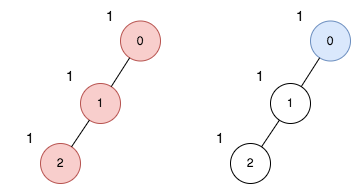
Input: n = 3, edges = [[0,1],[1,2]], price = [1,1,1]
Output: 2
Explanation: The diagram above denotes the tree after rooting it at node 0. The first part (colored in red) shows the path with the maximum price sum. The second part (colored in blue) shows the path with the minimum price sum.
- The first path contains nodes [0,1,2]: the prices are [1,1,1], and the sum of the prices is 3.
- The second path contains node [0] with a price [1].
The difference between the maximum and minimum price sum is 2. It can be proved that 2 is the maximum cost.
Constraints:
1 <= n <= 105edges.length == n - 10 <= ai, bi <= n - 1edges represents a valid tree.price.length == n1 <= price[i] <= 105Problem Overview: You are given a tree where each node has a price. Choose any node as the root. From that root, consider all paths that start at the root and end at some node in the tree. The score for that root is the difference between the maximum path price sum and the minimum path price sum. The task is to compute the maximum possible score across all choices of root.
Approach 1: DFS Based Path Sum Calculation (O(n) time, O(n) space)
The key observation is that the difference between maximum and minimum path sums can be transformed into a tree dynamic programming problem. During a Depth-First Search, track two values for every node: the best path sum that must end at a leaf in its subtree and the best path sum that can end at any node. These states allow you to model the minimum and maximum path choices. While traversing children, combine subtree results and update a global answer representing the best possible difference. This approach processes each edge once, making it linear time.
Implementation builds an adjacency list for the tree, then runs a recursive DFS. Each recursive call returns the best downward sums for the current node. While merging results from different children, compute candidate differences by pairing paths that represent the minimum-side constraint (ending at a leaf) and the maximum-side freedom (ending anywhere). The algorithm is essentially a tree DP with two states per node.
Approach 2: Centroid Decomposition (O(n log n) time, O(n) space)
Centroid decomposition treats the tree as a hierarchy of balanced components. At each centroid, compute path sums from the centroid into each subtree using DFS. By aggregating subtree results and comparing maximum and minimum path contributions, you can evaluate candidate differences that pass through the centroid. After processing, remove the centroid and recursively process the remaining components.
This method is useful when problems involve path queries or combinations of paths across different subtrees. Each level of decomposition handles paths that pass through a particular centroid, ensuring no path is processed more than O(log n) times overall. Although more complex than the DFS DP approach, it generalizes well for many advanced tree path problems.
Recommended for interviews: The DFS-based tree dynamic programming solution. It runs in O(n) time, requires only one traversal, and demonstrates strong understanding of path aggregation in trees. Centroid decomposition is powerful but usually unnecessary unless the interviewer explicitly pushes toward advanced tree techniques.
This approach involves using Depth-First Search (DFS) to traverse the tree and calculate the price sum paths for each node. The idea is to first perform a DFS from an arbitrary root to calculate the maximum path sum for each node as both the starting and ending node of a path. Using these precomputed values, the difference between maximum and minimum path sums can be computed efficiently by trying each node as a root one by one and tracking the possible maximum cost.
This solution utilizes two DFS traversals. In the first DFS, starting from an arbitrary node, it determines the farthest node and uses this farthest node as a starting point for calculating maximum path sums. In the second DFS, it calculates the maximum and minimum paths for each node when it acts as a root. After this pre-computation, the solution iterates through each node to determine the maximum possible cost.
Time Complexity: O(n), because each node and edge is visited a constant number of times in the DFS traversals.
Space Complexity: O(n), due to the recursive stack space and additional arrays for storing maximum and minimum path sums.
In this approach, centroid decomposition is employed for solving the problem more efficiently. The tree is considered recursively split at its centroid. This method helps efficiently calculate the price sums for paths without recalculating them from scratch for each potential root. In centroid decomposition, subproblems are solved and combined to achieve the global solution, and paths are calculated only once per component.
This involves calculating node sizes to find a centroid, breaking the tree at this centroid, and recursively processing each segment to evaluate costs. This decomposition minimizes repeated path calculations by using the tree’s structural properties.
Time Complexity: O(n log n), because each decomposition potentially halves the problem.
Space Complexity: O(n), attributed to additional data structures for centroid cut maintenance.
| Approach | Complexity |
|---|---|
| DFS Based Path Sum Calculation | Time Complexity: O(n), because each node and edge is visited a constant number of times in the DFS traversals. |
| Centroid Decomposition | Time Complexity: O(n log n), because each decomposition potentially halves the problem. |
| Default Approach | — |
| Approach | Time | Space | When to Use |
|---|---|---|---|
| DFS Based Path Sum Calculation | O(n) | O(n) | Best general solution for trees; single DFS with tree DP states |
| Centroid Decomposition | O(n log n) | O(n) | Useful for complex path aggregation problems or reusable centroid frameworks |
In Out DFS | Difference Between Maximum and Minimum Price Sum | Weekly Contest 328 • codingMohan • 3,036 views views
Watch 9 more video solutions →Practice Difference Between Maximum and Minimum Price Sum with our built-in code editor and test cases.
Practice on FleetCodePractice this problem
Open in Editor