There are n cities connected by some number of flights. You are given an array flights where flights[i] = [fromi, toi, pricei] indicates that there is a flight from city fromi to city toi with cost pricei.
You are also given three integers src, dst, and k, return the cheapest price from src to dst with at most k stops. If there is no such route, return -1.
Example 1:
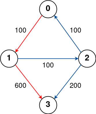
Input: n = 4, flights = [[0,1,100],[1,2,100],[2,0,100],[1,3,600],[2,3,200]], src = 0, dst = 3, k = 1
Output: 700
Explanation:
The graph is shown above.
The optimal path with at most 1 stop from city 0 to 3 is marked in red and has cost 100 + 600 = 700.
Note that the path through cities [0,1,2,3] is cheaper but is invalid because it uses 2 stops.
Example 2:
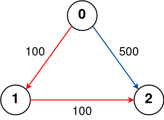
Input: n = 3, flights = [[0,1,100],[1,2,100],[0,2,500]], src = 0, dst = 2, k = 1
Output: 200
Explanation:
The graph is shown above.
The optimal path with at most 1 stop from city 0 to 2 is marked in red and has cost 100 + 100 = 200.
Example 3:
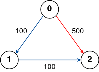
Input: n = 3, flights = [[0,1,100],[1,2,100],[0,2,500]], src = 0, dst = 2, k = 0
Output: 500
Explanation:
The graph is shown above.
The optimal path with no stops from city 0 to 2 is marked in red and has cost 500.
Constraints:
1 <= n <= 1000 <= flights.length <= (n * (n - 1) / 2)flights[i].length == 30 <= fromi, toi < nfromi != toi1 <= pricei <= 1040 <= src, dst, k < nsrc != dstProblem Overview: You are given n cities connected by flights where each edge has a price. The task is to find the cheapest cost from src to dst using at most k stops. The challenge is balancing shortest-path logic with a constraint on the number of intermediate nodes.
Approach 1: Breadth-First Search with Cost Tracking (Time: O(E * K), Space: O(V + E))
This approach treats the graph as levels of stops and explores it using Breadth-First Search. Build an adjacency list from the flights array, then perform BFS where each level represents one additional stop. Maintain the current cost to each node and only continue exploring if the new path is cheaper than previously recorded costs. The key insight is limiting traversal depth to k + 1 edges while pruning expensive paths early. This keeps exploration efficient even if the graph has many connections.
Approach 2: Dijkstra's Algorithm with Stop Constraint (Time: O(E log (V * K)), Space: O(V * K))
This method adapts shortest path logic using a min-heap (priority queue). Instead of storing only the node and cost, the state also tracks how many stops were used to reach the node. The heap always expands the cheapest path first. When a node is popped, its neighbors are pushed with updated cost and stop count, as long as the stop limit has not been exceeded. This guarantees the cheapest valid route is discovered early and works well when flight graphs are dense.
Recommended for interviews: Interviewers usually expect the Dijkstra-style solution because it directly models the constrained shortest-path problem and demonstrates familiarity with priority queues. Starting with the BFS idea shows you understand graph traversal with level constraints, but implementing the heap-based approach shows stronger mastery of graph optimization techniques.
In this approach, use BFS to explore all possible paths. Utilize a queue to store the current node, accumulated cost, and the number of stops made so far. The key is to traverse by layer, effectively managing the permitted stops through levels of BFS. If we reach the destination within the allowed stops, track the minimum cost.
This solution constructs a graph from the flights list using an adjacency list. For BFS, a queue keeps track of the current city, the accumulated cost to reach that city, and the number of remaining stops allowed. Traverse each city, and only append a city to the queue if doing so reduces the cost to reach it. This ensures we explore the cheapest path first, within k stops. The process continues until all nodes are explored or the cheapest path is found.
Python
JavaScript
Time Complexity: O(n * k) in the worst case when every city is connected.
Space Complexity: O(n) for storing the graph and queue.
This approach leverages a modified version of Dijkstra's algorithm to explore paths from source to destination using a prioritized data structure like a min-heap. Each entry tracks not only the cumulative cost but also the number of stops taken. The algorithm ensures the shortest paths are evaluated first and skips any path with exceeding stops, thus efficiently finding the minimum cost path within allowed stops.
This C++ solution utilizes a min-heap or priority queue data structure to maintain the current city, accumulated cost, and stops left. Priority ensures that cities with the smallest accumulated cost are processed first, following Dijkstra's logic but capped by the number of stops. Each step examines the target city, updating the cost and queuing potential paths until either the destination is reached within allowed stops or the queue is exhausted.
Time Complexity: O((n+k) log n) reflects edge processing and heap operations.
Space Complexity: O(n) taken by the adjacency list and tracking structures.
| Approach | Complexity |
|---|---|
| Breadth-First Search (BFS) with Cost Tracking | Time Complexity: O(n * k) in the worst case when every city is connected. |
| Dijkstra's Algorithm Adaptation | Time Complexity: O((n+k) log n) reflects edge processing and heap operations. |
| Default Approach | — |
| Approach | Time | Space | When to Use |
|---|---|---|---|
| BFS with Cost Tracking | O(E * K) | O(V + E) | When the stop limit is small and you want a simple level-based traversal. |
| Dijkstra with Stop Constraint | O(E log (V * K)) | O(V * K) | General case for weighted graphs where the cheapest path must respect stop limits. |
G-38. Cheapest Flights Within K Stops • take U forward • 312,097 views views
Watch 9 more video solutions →Practice Cheapest Flights Within K Stops with our built-in code editor and test cases.
Practice on FleetCode