Given the root of a binary tree, calculate the vertical order traversal of the binary tree.
For each node at position (row, col), its left and right children will be at positions (row + 1, col - 1) and (row + 1, col + 1) respectively. The root of the tree is at (0, 0).
The vertical order traversal of a binary tree is a list of top-to-bottom orderings for each column index starting from the leftmost column and ending on the rightmost column. There may be multiple nodes in the same row and same column. In such a case, sort these nodes by their values.
Return the vertical order traversal of the binary tree.
Example 1:
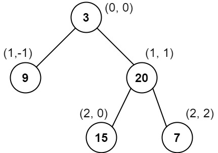
Input: root = [3,9,20,null,null,15,7]
Output: [[9],[3,15],[20],[7]]
Explanation:
Column -1: Only node 9 is in this column.
Column 0: Nodes 3 and 15 are in this column in that order from top to bottom.
Column 1: Only node 20 is in this column.
Column 2: Only node 7 is in this column.
Example 2:

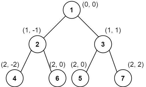
Input: root = [1,2,3,4,5,6,7]
Output: [[4],[2],[1,5,6],[3],[7]]
Explanation:
Column -2: Only node 4 is in this column.
Column -1: Only node 2 is in this column.
Column 0: Nodes 1, 5, and 6 are in this column.
          1 is at the top, so it comes first.
          5 and 6 are at the same position (2, 0), so we order them by their value, 5 before 6.
Column 1: Only node 3 is in this column.
Column 2: Only node 7 is in this column.
Example 3:
Input: root = [1,2,3,4,6,5,7]
Output: [[4],[2],[1,5,6],[3],[7]]
Explanation:
This case is the exact same as example 2, but with nodes 5 and 6 swapped.
Note that the solution remains the same since 5 and 6 are in the same location and should be ordered by their values.
Constraints:
[1, 1000].0 <= Node.val <= 1000Problem Overview: You are given the root of a binary tree and need to return its vertical order traversal. Each node is assigned coordinates: the root starts at column 0, left child moves to col - 1, and right child moves to col + 1. Nodes must be grouped by column from left to right. If multiple nodes share the same row and column, they must be ordered by their values.
Approach 1: BFS with Coordinate Tracking (Time: O(n log n), Space: O(n))
This approach performs a level-order traversal using a queue while tracking each node’s (row, column) coordinates. Start with the root at (0,0). When visiting a node, push its children into the queue with updated coordinates: left child (row+1, col-1) and right child (row+1, col+1). Store nodes in a hash map where the key is the column and the value is a list of (row, value) pairs. After traversal, sort each column’s entries first by row and then by value to satisfy the ordering constraint. Finally, iterate columns from the minimum to maximum index to build the result. This method is intuitive because Breadth-First Search naturally processes nodes level by level, making row tracking straightforward.
Approach 2: DFS with Sorting (Time: O(n log n), Space: O(n))
This solution uses recursive traversal to record the position of every node. During the DFS, pass the current row and column values to children and store tuples (column, row, value) in a list. After visiting all nodes, sort the list primarily by column, then by row, and finally by node value. Once sorted, iterate through the list and group nodes with the same column together. The advantage of this approach is its simplicity: all ordering logic is handled by a single sort operation. It combines Depth-First Search traversal with a sorting step to enforce the problem’s ordering rules.
Recommended for interviews: BFS with coordinate tracking is usually easier to reason about during interviews because it mirrors the grid-like interpretation of the tree. You explicitly track positions and group nodes by column using a hash table. DFS with sorting is equally valid and often shorter to implement, but interviewers typically expect you to explain how row and column ordering are preserved. Showing the coordinate idea first demonstrates strong problem modeling, while the optimized grouping and sorting show implementation skill.
This approach uses a Breadth-First Search (BFS) to traverse the tree while tracking each node's position (row, col). We use a queue to manage our BFS process, which stores tuples of (node, row, col). As we visit each node, we place it into a list corresponding to its column index. Finally, we sort each column by first row, then value, and construct the result.
We initialize a queue for BFS, starting with the root node at position (0, 0). For each node processed, we record its value in a list corresponding to its column index and adjust column bounds.
Finally, for each column, we sort the nodes first by their row and then by value, assembling the output in column order. This efficiently manages the node organization for vertical traversal.
Time Complexity: O(N log N) due to sorting, where N is the number of nodes.
Space Complexity: O(N) for the storage of node values, where N is the number of nodes.
This method involves performing a pre-order traversal (DFS) to collect all nodes along with their column and row indices. Once collected, nodes are sorted based on their columns first, then their rows, and finally their values. The sorted list is then grouped into lists according to their column indices to produce the final vertical order traversal.
The DFS collects nodes with their positions into a list. This unsorted list is then sorted by column, row, and value. Finally, nodes are classified into their corresponding columns based on sorted order.
This approach relies on sorting all nodes at the end to define their order in the result.
Time Complexity: O(N log N) due to sorting, where N is the total number of nodes.
Space Complexity: O(N) to store all the nodes along with their positions.
We design a function dfs(root, i, j), where i and j represent the row and column of the current node. We can record the row and column information of the nodes through depth-first search, store it in an array or list nodes, and then sort nodes in the order of column, row, and value.
Next, we traverse nodes, putting the values of nodes in the same column into the same list, and finally return these lists.
The time complexity is O(n times log n), and the space complexity is O(n). Here, n is the number of nodes in the binary tree.
Python
Java
C++
Go
TypeScript
| Approach | Complexity |
|---|---|
| Approach 1: BFS with Coordinate Tracking | Time Complexity: O(N log N) due to sorting, where N is the number of nodes. Space Complexity: O(N) for the storage of node values, where N is the number of nodes. |
| Approach 2: DFS with Sorting | Time Complexity: O(N log N) due to sorting, where N is the total number of nodes. Space Complexity: O(N) to store all the nodes along with their positions. |
| DFS + Sorting | — |
| Approach | Time | Space | When to Use |
|---|---|---|---|
| BFS with Coordinate Tracking | O(n log n) | O(n) | Best for interview explanations and when modeling nodes by grid coordinates. |
| DFS with Sorting | O(n log n) | O(n) | Simpler implementation when you prefer collecting all nodes then sorting once. |
Vertical order traversal of a binary tree | Leetcode #987 • Techdose • 58,662 views views
Watch 9 more video solutions →Practice Vertical Order Traversal of a Binary Tree with our built-in code editor and test cases.
Practice on FleetCode