Watch 2 video solutions for Number of Ways to Assign Edge Weights II, a hard level problem involving Array, Math, Dynamic Programming. This walkthrough by Programming Live with Larry has 253 views views. Want to try solving it yourself? Practice on FleetCode or read the detailed text solution.
There is an undirected tree with n nodes labeled from 1 to n, rooted at node 1. The tree is represented by a 2D integer array edges of length n - 1, where edges[i] = [ui, vi] indicates that there is an edge between nodes ui and vi.
Initially, all edges have a weight of 0. You must assign each edge a weight of either 1 or 2.
The cost of a path between any two nodes u and v is the total weight of all edges in the path connecting them.
You are given a 2D integer array queries. For each queries[i] = [ui, vi], determine the number of ways to assign weights to edges in the path such that the cost of the path between ui and vi is odd.
Return an array answer, where answer[i] is the number of valid assignments for queries[i].
Since the answer may be large, apply modulo 109 + 7 to each answer[i].
Note: For each query, disregard all edges not in the path between node ui and vi.
Example 1:
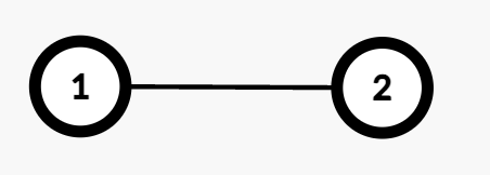
Input: edges = [[1,2]], queries = [[1,1],[1,2]]
Output: [0,1]
Explanation:
[1,1]: The path from Node 1 to itself consists of no edges, so the cost is 0. Thus, the number of valid assignments is 0.[1,2]: The path from Node 1 to Node 2 consists of one edge (1 → 2). Assigning weight 1 makes the cost odd, while 2 makes it even. Thus, the number of valid assignments is 1.Example 2:
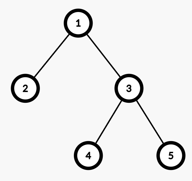
Input: edges = [[1,2],[1,3],[3,4],[3,5]], queries = [[1,4],[3,4],[2,5]]
Output: [2,1,4]
Explanation:
[1,4]: The path from Node 1 to Node 4 consists of two edges (1 → 3 and 3 → 4). Assigning weights (1,2) or (2,1) results in an odd cost. Thus, the number of valid assignments is 2.[3,4]: The path from Node 3 to Node 4 consists of one edge (3 → 4). Assigning weight 1 makes the cost odd, while 2 makes it even. Thus, the number of valid assignments is 1.[2,5]: The path from Node 2 to Node 5 consists of three edges (2 → 1, 1 → 3, and 3 → 5). Assigning (1,2,2), (2,1,2), (2,2,1), or (1,1,1) makes the cost odd. Thus, the number of valid assignments is 4.
Constraints:
2 <= n <= 105edges.length == n - 1edges[i] == [ui, vi]1 <= queries.length <= 105queries[i] == [ui, vi]1 <= ui, vi <= nedges represents a valid tree.Problem Overview: You are given a tree and must assign weights to its edges while satisfying specific constraints defined by the problem. The task is to count how many valid assignments exist. Because the structure is a tree, the solution relies heavily on depth-first traversal and dynamic programming to combine valid configurations from child subtrees.
Approach 1: Brute Force Edge Assignment (Exponential Time)
The most direct idea is to try every possible weight assignment for every edge and check whether the resulting configuration satisfies the constraints. With n-1 edges, even a small number of possible weights leads to exponential combinations. After assigning weights, you validate the tree by traversing it and verifying the conditions. This approach has O(k^(n)) time complexity where k is the number of possible weights, and O(n) space for traversal state. It works only for very small inputs and mainly serves as a conceptual baseline.
Approach 2: Tree Dynamic Programming with DFS (Optimal)
The efficient strategy uses Depth-First Search to process the tree from the root while maintaining dynamic programming states for each subtree. For every node, you compute how many valid assignments exist for the subtree depending on the state propagated from its parent edge. Each child contributes a set of valid configurations, and the parent combines them using multiplication or state transitions.
Bit manipulation helps encode constraint states efficiently. For example, if the validity of assignments depends on parity or bitwise conditions along a path, you represent those properties using a bitmask and update them while traversing edges. This keeps transitions constant time and avoids recomputation. The DFS aggregates results from children and stores them in a DP table per node.
This approach runs in O(n * s) time where s is the number of possible DP states derived from the bitmask or constraint representation. Space complexity is O(n * s) for storing DP states across the tree. The method combines ideas from Dynamic Programming, Tree algorithms, and bitmask state compression.
Recommended for interviews: Interviewers expect the tree DP approach with DFS. Starting with the brute force explanation shows you understand the search space, but recognizing that the tree structure allows state aggregation from children demonstrates strong algorithmic reasoning.
| Approach | Time | Space | When to Use |
|---|---|---|---|
| Brute Force Edge Assignment | O(k^n) | O(n) | Useful only for very small trees or reasoning about the search space |
| Tree DP with DFS and Bitmask States | O(n * s) | O(n * s) | General case; scalable for large trees with constrained state transitions |