Watch 10 video solutions for Minimum Path Cost in a Grid, a medium level problem involving Array, Dynamic Programming, Matrix. This walkthrough by Coding Decoded has 2,868 views views. Want to try solving it yourself? Practice on FleetCode or read the detailed text solution.
You are given a 0-indexed m x n integer matrix grid consisting of distinct integers from 0 to m * n - 1. You can move in this matrix from a cell to any other cell in the next row. That is, if you are in cell (x, y) such that x < m - 1, you can move to any of the cells (x + 1, 0), (x + 1, 1), ..., (x + 1, n - 1). Note that it is not possible to move from cells in the last row.
Each possible move has a cost given by a 0-indexed 2D array moveCost of size (m * n) x n, where moveCost[i][j] is the cost of moving from a cell with value i to a cell in column j of the next row. The cost of moving from cells in the last row of grid can be ignored.
The cost of a path in grid is the sum of all values of cells visited plus the sum of costs of all the moves made. Return the minimum cost of a path that starts from any cell in the first row and ends at any cell in the last row.
Example 1:
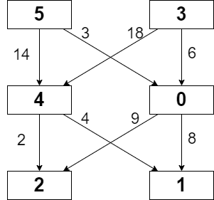
Input: grid = [[5,3],[4,0],[2,1]], moveCost = [[9,8],[1,5],[10,12],[18,6],[2,4],[14,3]]
Output: 17
Explanation: The path with the minimum possible cost is the path 5 -> 0 -> 1.
- The sum of the values of cells visited is 5 + 0 + 1 = 6.
- The cost of moving from 5 to 0 is 3.
- The cost of moving from 0 to 1 is 8.
So the total cost of the path is 6 + 3 + 8 = 17.
Example 2:
Input: grid = [[5,1,2],[4,0,3]], moveCost = [[12,10,15],[20,23,8],[21,7,1],[8,1,13],[9,10,25],[5,3,2]]
Output: 6
Explanation: The path with the minimum possible cost is the path 2 -> 3.
- The sum of the values of cells visited is 2 + 3 = 5.
- The cost of moving from 2 to 3 is 1.
So the total cost of this path is 5 + 1 = 6.
Constraints:
m == grid.lengthn == grid[i].length2 <= m, n <= 50grid consists of distinct integers from 0 to m * n - 1.moveCost.length == m * nmoveCost[i].length == n1 <= moveCost[i][j] <= 100Problem Overview: You are given a grid where you start from any cell in the first row and move down one row at a time. Moving from value v to column c in the next row adds an extra cost from the moveCost[v][c] table. The goal is to reach the last row with the minimum total cost including both cell values and movement costs.
Approach 1: Dynamic Programming (O(m * n^2) time, O(m * n) space)
The natural way to solve this is bottom-up dynamic programming. Define dp[r][c] as the minimum cost to reach cell (r, c). Initialize the first row with the grid values because you can start from any column. For every cell in row r, iterate over all columns in row r + 1 and update the transition using dp[r][c] + moveCost[grid[r][c]][nextCol] + grid[r+1][nextCol]. This effectively tries every valid downward move and keeps the minimum cost. Since each of the m * n cells can transition to n columns in the next row, the time complexity becomes O(m * n^2) with O(m * n) space (or O(n) with row compression). This approach directly models the problem and is the most common solution in interviews involving matrix transitions.
Approach 2: Greedy with Priority Queue (Dijkstra-style) (O(m * n^2 log(mn)) time, O(m * n) space)
You can also treat the grid as a weighted graph. Each cell (r, c) is a node, and it has edges to every cell in row r + 1. The edge weight equals moveCost[grid[r][c]][nextCol] + grid[r+1][nextCol]. Start by pushing all first-row cells into a min-heap with their grid values as initial costs. Then repeatedly pop the smallest cost state and relax edges to the next row using a priority queue from array-based grid positions. This behaves like Dijkstra's shortest path algorithm. The heap ensures the next processed state always has the smallest accumulated cost. Because each node may push up to n transitions and heap operations cost log(mn), the total complexity is O(m * n^2 log(mn)).
Recommended for interviews: The dynamic programming solution is what most interviewers expect. The grid naturally forms layered states (row by row), making the DP transition straightforward and easy to reason about. Mentioning the graph interpretation shows deeper understanding, but implementing DP with a clear transition and optionally compressing to O(n) space demonstrates stronger problem-solving skill.
| Approach | Time | Space | When to Use |
|---|---|---|---|
| Dynamic Programming | O(m * n^2) | O(m * n) or O(n) | Best general solution. Directly models row-to-row transitions and is easy to implement in interviews. |
| Greedy with Priority Queue (Dijkstra) | O(m * n^2 log(mn)) | O(m * n) | Useful when thinking of the grid as a weighted graph or when applying shortest path algorithms. |