
Minimum Path Cost in a Grid - Solution & Explanation
Problem Statement
You are given a 0-indexed m x n integer matrix grid consisting of distinct integers from 0 to m * n - 1. You can move in this matrix from a cell to any other cell in the next row. That is, if you are in cell (x, y) such that x < m - 1, you can move to any of the cells (x + 1, 0), (x + 1, 1), ..., (x + 1, n - 1). Note that it is not possible to move from cells in the last row.
Each possible move has a cost given by a 0-indexed 2D array moveCost of size (m * n) x n, where moveCost[i][j] is the cost of moving from a cell with value i to a cell in column j of the next row. The cost of moving from cells in the last row of grid can be ignored.
The cost of a path in grid is the sum of all values of cells visited plus the sum of costs of all the moves made. Return the minimum cost of a path that starts from any cell in the first row and ends at any cell in the last row.
Example 1:
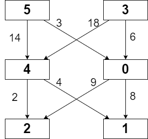
Input: grid = [[5,3],[4,0],[2,1]], moveCost = [[9,8],[1,5],[10,12],[18,6],[2,4],[14,3]]
Output: 17
Explanation: The path with the minimum possible cost is the path 5 -> 0 -> 1.
- The sum of the values of cells visited is 5 + 0 + 1 = 6.
- The cost of moving from 5 to 0 is 3.
- The cost of moving from 0 to 1 is 8.
So the total cost of the path is 6 + 3 + 8 = 17.
Example 2:
Input: grid = [[5,1,2],[4,0,3]], moveCost = [[12,10,15],[20,23,8],[21,7,1],[8,1,13],[9,10,25],[5,3,2]]
Output: 6
Explanation: The path with the minimum possible cost is the path 2 -> 3.
- The sum of the values of cells visited is 2 + 3 = 5.
- The cost of moving from 2 to 3 is 1.
So the total cost of this path is 5 + 1 = 6.
Constraints:
m == grid.lengthn == grid[i].length2 <= m, n <= 50gridconsists of distinct integers from0tom * n - 1.moveCost.length == m * nmoveCost[i].length == n1 <= moveCost[i][j] <= 100
Approach Overview
Problem Overview: You are given a grid where you start from any cell in the first row and move down one row at a time. Moving from value v to column c in the next row adds an extra cost from the moveCost[v][c] table. The goal is to reach the last row with the minimum total cost including both cell values and movement costs.
Approach 1: Dynamic Programming (O(m * n^2) time, O(m * n) space)
The natural way to solve this is bottom-up dynamic programming. Define dp[r][c] as the minimum cost to reach cell (r, c). Initialize the first row with the grid values because you can start from any column. For every cell in row r, iterate over all columns in row r + 1 and update the transition using dp[r][c] + moveCost[grid[r][c]][nextCol] + grid[r+1][nextCol]. This effectively tries every valid downward move and keeps the minimum cost. Since each of the m * n cells can transition to n columns in the next row, the time complexity becomes O(m * n^2) with O(m * n) space (or O(n) with row compression). This approach directly models the problem and is the most common solution in interviews involving matrix transitions.
Approach 2: Greedy with Priority Queue (Dijkstra-style) (O(m * n^2 log(mn)) time, O(m * n) space)
You can also treat the grid as a weighted graph. Each cell (r, c) is a node, and it has edges to every cell in row r + 1. The edge weight equals moveCost[grid[r][c]][nextCol] + grid[r+1][nextCol]. Start by pushing all first-row cells into a min-heap with their grid values as initial costs. Then repeatedly pop the smallest cost state and relax edges to the next row using a priority queue from array-based grid positions. This behaves like Dijkstra's shortest path algorithm. The heap ensures the next processed state always has the smallest accumulated cost. Because each node may push up to n transitions and heap operations cost log(mn), the total complexity is O(m * n^2 log(mn)).
Recommended for interviews: The dynamic programming solution is what most interviewers expect. The grid naturally forms layered states (row by row), making the DP transition straightforward and easy to reason about. Mentioning the graph interpretation shows deeper understanding, but implementing DP with a clear transition and optionally compressing to O(n) space demonstrates stronger problem-solving skill.
Approach 1: Dynamic Programming Approach
In this approach, we use a dynamic programming table (often referred to as dp) to store the minimum cost to reach a cell in the grid from any cell in the previous row. The solution involves filling up this dp table row by row, using previously computed values to calculate the current values.
The code initializes a dp array for storing the minimum path cost to reach each cell in the grid. It iterates through each row, updating this array based on the possible moves considering the moveCost and the current grid values.
Complexity
Time complexity is O(m * n^2) due to the nested loops, and space complexity is O(n), where m is the number of rows and n is the number of columns.
Approach 2: Greedy Approach with Priority Queue
This approach uses a priority queue (min-heap) to greedily explore paths with the least cost first. By maintaining a priority queue arranged by path costs, we can always expand the shortest path first, ensuring the minimum cost path is found efficiently.
This Python implementation uses a priority queue (using the heapq module) to maintain paths by their cumulative cost. By always expanding the path with the smallest cost first, it ensures that we find the minimum cost path optimally.
Code
Python
Complexity
Time complexity: O(m * n log n); Space complexity: O(m * n).
Approach 3: Dynamic Programming
We define f[i][j] to represent the minimum path cost from the first row to the ith row and jth column. Since we can only move from a column in the previous row to a column in the current row, the value of f[i][j] can be transferred from f[i - 1][k], where the range of k is [0, n - 1]. Therefore, the state transition equation is:
$
f[i][j] = min_{0 leq k < n} {f[i - 1][k] + moveCost[grid[i - 1][k]][j] + grid[i][j]}
where moveCost[grid[i - 1][k]][j] represents the cost of moving from the kth column of the i - 1th row to the jth column of the ith row.
The final answer is min_{0 leq j < n} {f[m - 1][j]}.
Since each transition only needs the state of the previous row, we can use a rolling array to optimize the space complexity to O(n).
The time complexity is O(m times n^2), and the space complexity is O(n). Here, m and n$ are the number of rows and columns of the grid, respectively.
Complexity Comparison
| Approach | Complexity |
|---|---|
| Dynamic Programming Approach | Time complexity is O(m * n^2) due to the nested loops, and space complexity is O(n), where m is the number of rows and n is the number of columns. |
| Greedy Approach with Priority Queue | Time complexity: O(m * n log n); Space complexity: O(m * n). |
| Dynamic Programming | — |
Detailed Complexity Analysis
| Approach | Time | Space | When to Use |
|---|---|---|---|
| Dynamic Programming | O(m * n^2) | O(m * n) or O(n) | Best general solution. Directly models row-to-row transitions and is easy to implement in interviews. |
| Greedy with Priority Queue (Dijkstra) | O(m * n^2 log(mn)) | O(m * n) | Useful when thinking of the grid as a weighted graph or when applying shortest path algorithms. |
Video Solution
Weekly Contest 297| Leetcode 2303 2304 2305 |Minimum Path Cost in a Grid| Fair Distribution Cookies • Coding Decoded • 2,899 views views
Watch 8 more video solutions →Frequently Asked Questions
Is Minimum Path Cost in a Grid easy or hard?
Minimum Path Cost in a Grid Python or Java solution
How to solve Minimum Path Cost in a Grid in O(m * n^2)?
What is the best approach for Minimum Path Cost in a Grid?
What data structure is used in Minimum Path Cost in a Grid?
What is the time complexity of Minimum Path Cost in a Grid?
Is Minimum Path Cost in a Grid asked at Google, Amazon, or Meta?
Ready to solve this problem?
Practice Minimum Path Cost in a Grid with our built-in code editor and test cases.
Practice on FleetCode