Watch 10 video solutions for Minimum Cost to Make at Least One Valid Path in a Grid, a hard level problem involving Array, Breadth-First Search, Graph. This walkthrough by NeetCodeIO has 13,077 views views. Want to try solving it yourself? Practice on FleetCode or read the detailed text solution.
Given an m x n grid. Each cell of the grid has a sign pointing to the next cell you should visit if you are currently in this cell. The sign of grid[i][j] can be:
1 which means go to the cell to the right. (i.e go from grid[i][j] to grid[i][j + 1])2 which means go to the cell to the left. (i.e go from grid[i][j] to grid[i][j - 1])3 which means go to the lower cell. (i.e go from grid[i][j] to grid[i + 1][j])4 which means go to the upper cell. (i.e go from grid[i][j] to grid[i - 1][j])Notice that there could be some signs on the cells of the grid that point outside the grid.
You will initially start at the upper left cell (0, 0). A valid path in the grid is a path that starts from the upper left cell (0, 0) and ends at the bottom-right cell (m - 1, n - 1) following the signs on the grid. The valid path does not have to be the shortest.
You can modify the sign on a cell with cost = 1. You can modify the sign on a cell one time only.
Return the minimum cost to make the grid have at least one valid path.
Example 1:
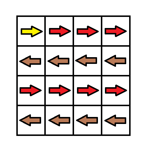
Input: grid = [[1,1,1,1],[2,2,2,2],[1,1,1,1],[2,2,2,2]]
Output: 3
Explanation: You will start at point (0, 0).
The path to (3, 3) is as follows. (0, 0) --> (0, 1) --> (0, 2) --> (0, 3) change the arrow to down with cost = 1 --> (1, 3) --> (1, 2) --> (1, 1) --> (1, 0) change the arrow to down with cost = 1 --> (2, 0) --> (2, 1) --> (2, 2) --> (2, 3) change the arrow to down with cost = 1 --> (3, 3)
The total cost = 3.
Example 2:
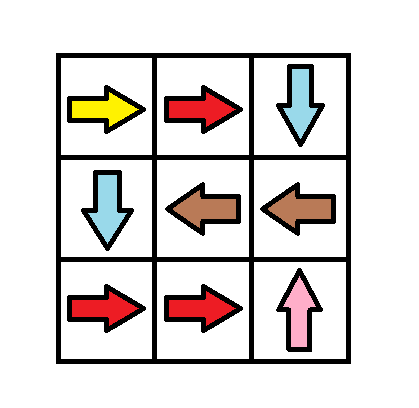
Input: grid = [[1,1,3],[3,2,2],[1,1,4]]
Output: 0
Explanation: You can follow the path from (0, 0) to (2, 2).
Example 3:
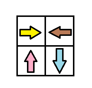
Input: grid = [[1,2],[4,3]]
Output: 1
Constraints:
m == grid.lengthn == grid[i].length1 <= m, n <= 1001 <= grid[i][j] <= 4Problem Overview: You get an m x n grid where each cell contains a direction (right, left, down, up). Following the direction costs 0, but changing it costs 1. The goal is to reach the bottom-right cell from the top-left with the minimum total modification cost.
The grid naturally forms a directed graph: every cell has an outgoing edge based on its arrow. Moving in the indicated direction costs 0, while moving to any other neighbor requires paying 1 to change the sign. The task becomes a classic shortest path problem on a weighted grid graph.
Approach 1: Dijkstra-like BFS Using Priority Queue (O(mn log(mn)) time, O(mn) space)
Treat each cell as a node in a graph and run Dijkstra’s algorithm. From each position, explore the four neighbors. If the move matches the arrow in the current cell, the cost stays the same; otherwise add 1. A min-heap (priority queue) always expands the cell with the lowest accumulated cost. Maintain a dist matrix to store the minimum cost seen for each cell and skip states that are already improved. This works because all edge weights are non‑negative. The algorithm guarantees the first time you pop the destination from the heap, you have the optimal cost.
This method is essentially shortest path on a graph represented by a matrix. It is the most intuitive approach when you recognize the weighted edges. Works well even for the largest constraints.
Approach 2: Bellman-Ford-like Relaxation (O(mn * 4 * iterations) time, O(mn) space)
Instead of using a priority queue, repeatedly relax edges across the grid. Initialize the cost of the start cell as 0 and all others as infinity. For each cell, check its four neighbors and update their cost using the same rule: +0 if the arrow matches, +1 otherwise. Continue relaxing until no updates occur or until the grid stabilizes. This mirrors the Bellman-Ford process of relaxing edges until shortest paths converge.
This version is easier to implement in languages where priority queues are slower or when you want a straightforward dynamic relaxation loop. It still models the problem as a shortest-path computation but without the heap optimization.
Conceptually, both approaches rely on graph traversal and shortest path relaxation techniques. Understanding how the grid becomes a graph is key. Many candidates also frame the optimal solution as a variation of Breadth-First Search where zero-cost edges are prioritized.
Recommended for interviews: The Dijkstra-like BFS with a priority queue is the expected solution. It clearly models the grid as a weighted graph and runs in O(mn log(mn)). Explaining the relaxation idea first shows you understand shortest-path fundamentals, while implementing the heap-based solution demonstrates practical algorithm skill.
| Approach | Time | Space | When to Use |
|---|---|---|---|
| Dijkstra-like BFS with Priority Queue | O(mn log(mn)) | O(mn) | Best general solution for weighted grid shortest path problems |
| Bellman-Ford-style Relaxation | O(mn * iterations) | O(mn) | Simpler implementation when repeatedly relaxing edges without a heap |