Watch 10 video solutions for Maximum Width of Binary Tree, a medium level problem involving Tree, Depth-First Search, Breadth-First Search. This walkthrough by take U forward has 433,240 views views. Want to try solving it yourself? Practice on FleetCode or read the detailed text solution.
Given the root of a binary tree, return the maximum width of the given tree.
The maximum width of a tree is the maximum width among all levels.
The width of one level is defined as the length between the end-nodes (the leftmost and rightmost non-null nodes), where the null nodes between the end-nodes that would be present in a complete binary tree extending down to that level are also counted into the length calculation.
It is guaranteed that the answer will in the range of a 32-bit signed integer.
Example 1:
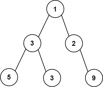
Input: root = [1,3,2,5,3,null,9]
Output: 4
Explanation: The maximum width exists in the third level with length 4 (5,3,null,9).
Example 2:
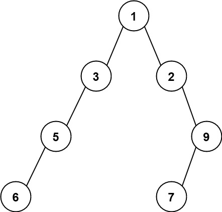
Input: root = [1,3,2,5,null,null,9,6,null,7]
Output: 7
Explanation: The maximum width exists in the fourth level with length 7 (6,null,null,null,null,null,7).
Example 3:
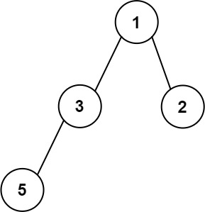
Input: root = [1,3,2,5]
Output: 2
Explanation: The maximum width exists in the second level with length 2 (3,2).
Constraints:
[1, 3000].-100 <= Node.val <= 100Problem Overview: You are given the root of a binary tree. The width of a level is defined as the distance between the leftmost and rightmost non-null nodes, counting the null positions that would exist in a complete binary tree. The task is to compute the maximum width across all levels.
Approach 1: Level Order Traversal with Position Tracking (O(n) time, O(n) space)
This approach performs a standard Breadth-First Search using a queue. Each node is assigned a positional index as if the tree were stored in an array representation of a complete binary tree. The root starts at index 0, the left child gets 2*i, and the right child gets 2*i + 1. For every level, record the index of the first and last node in the queue. The width of that level is last_index - first_index + 1. The algorithm iterates level by level, updating the maximum width seen so far.
This works because positional indices preserve the virtual gaps between nodes that would appear in a complete tree layout. Even if some nodes are missing, the index difference still captures the correct width. Since each node is processed exactly once, the traversal runs in O(n) time with O(n) queue space in the worst case.
Approach 2: DFS with Position Tracking (O(n) time, O(h) space)
A Depth-First Search can compute the same width by tracking the first index encountered at every depth. Traverse the binary tree recursively while passing two values: the current depth and the node's positional index. When visiting a depth for the first time, store that index as the leftmost position for that level. For every node visited later at the same depth, compute the width using current_index - first_index_at_depth + 1.
This approach avoids storing entire levels like BFS. Instead, it only stores the first index for each depth and relies on recursion to explore the tree. The maximum width is updated during traversal. Because each node is visited once, the time complexity remains O(n). Space complexity becomes O(h) for recursion depth, where h is the tree height (up to O(n) in skewed trees).
Recommended for interviews: The level-order BFS approach is the most common interview solution. It clearly demonstrates understanding of tree traversal and how to simulate complete-tree indexing. The DFS variant shows deeper insight and uses less auxiliary memory when the tree height is small. Showing BFS first and then mentioning DFS as an optimization signals strong problem-solving depth.
| Approach | Time | Space | When to Use |
|---|---|---|---|
| Level Order Traversal with Position Tracking (BFS) | O(n) | O(n) | Best general solution. Easy to reason about because width is computed level by level. |
| DFS with Position Tracking | O(n) | O(h) | Useful when avoiding large queues. Works well when tree height is relatively small. |