Watch 10 video solutions for Lowest Common Ancestor of a Binary Search Tree, a medium level problem involving Tree, Depth-First Search, Binary Search Tree. This walkthrough by NeetCode has 346,743 views views. Want to try solving it yourself? Practice on FleetCode or read the detailed text solution.
Given a binary search tree (BST), find the lowest common ancestor (LCA) node of two given nodes in the BST.
According to the definition of LCA on Wikipedia: “The lowest common ancestor is defined between two nodes p and q as the lowest node in T that has both p and q as descendants (where we allow a node to be a descendant of itself).”
Example 1:
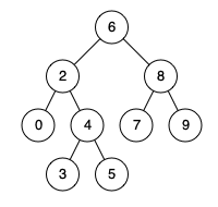
Input: root = [6,2,8,0,4,7,9,null,null,3,5], p = 2, q = 8
Output: 6
Explanation: The LCA of nodes 2 and 8 is 6.
Example 2:
Input: root = [6,2,8,0,4,7,9,null,null,3,5], p = 2, q = 4
Output: 2
Explanation: The LCA of nodes 2 and 4 is 2, since a node can be a descendant of itself according to the LCA definition.
Example 3:
Input: root = [2,1], p = 2, q = 1
Output: 2
Constraints:
[2, 105].-109 <= Node.val <= 109Node.val are unique.p != qp and q will exist in the BST.Problem Overview: Given a Binary Search Tree (BST) and two nodes p and q, return their lowest common ancestor (LCA). The LCA is the lowest node in the tree that has both nodes as descendants. Because the structure is a BST, every node follows the rule left < root < right, which allows you to locate the ancestor without scanning the entire tree.
Approach 1: Recursive BST Traversal (O(h) time, O(h) space)
The BST property gives a direct way to locate the ancestor. Start from the root and compare the values of p and q with the current node. If both values are smaller than the current node, the LCA must be in the left subtree. If both are larger, move to the right subtree. The first node where the values split (one on each side) is the lowest common ancestor. The recursion follows a single path from the root down the tree, so the time complexity is O(h), where h is the tree height, and recursion adds O(h) call stack space.
This approach naturally mirrors how you search in a Binary Search Tree. It is concise and easy to reason about during interviews because each recursive step eliminates half of the search space.
Approach 2: Iterative Traversal (O(h) time, O(1) space)
The iterative version applies the exact same BST insight but replaces recursion with a loop. Start from the root and repeatedly compare p.val and q.val with the current node value. If both are smaller, move to node.left. If both are larger, move to node.right. When the current node lies between the two values (or equals one of them), you have found the LCA.
This method walks down only one branch of the tree, so the time complexity remains O(h). Because it uses a simple pointer traversal instead of recursive calls, the space complexity improves to O(1). In balanced BSTs the height is O(log n), but in the worst case of a skewed tree it becomes O(n).
The approach relies heavily on the ordering guarantee of a tree that satisfies BST rules. Unlike general Depth-First Search LCA problems, you never need to explore both subtrees.
Recommended for interviews: The iterative BST traversal is usually the expected optimal solution because it runs in O(h) time with constant space. The recursive version still demonstrates a solid understanding of BST structure and is often written faster during interviews. Strong candidates quickly recognize that the BST ordering eliminates the need for full DFS or path tracking.
| Approach | Time | Space | When to Use |
|---|---|---|---|
| Recursive BST Traversal | O(h) | O(h) | When recursion is acceptable and you want concise logic that mirrors BST search |
| Iterative BST Traversal | O(h) | O(1) | Preferred for interviews or memory‑constrained environments since it avoids recursion stack |