Watch 10 video solutions for Count Pairs of Connectable Servers in a Weighted Tree Network, a medium level problem involving Array, Tree, Depth-First Search. This walkthrough by Aryan Mittal has 4,615 views views. Want to try solving it yourself? Practice on FleetCode or read the detailed text solution.
You are given an unrooted weighted tree with n vertices representing servers numbered from 0 to n - 1, an array edges where edges[i] = [ai, bi, weighti] represents a bidirectional edge between vertices ai and bi of weight weighti. You are also given an integer signalSpeed.
Two servers a and b are connectable through a server c if:
a < b, a != c and b != c.c to a is divisible by signalSpeed.c to b is divisible by signalSpeed.c to b and the path from c to a do not share any edges.Return an integer array count of length n where count[i] is the number of server pairs that are connectable through the server i.
Example 1:
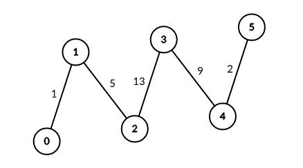
Input: edges = [[0,1,1],[1,2,5],[2,3,13],[3,4,9],[4,5,2]], signalSpeed = 1
Output: [0,4,6,6,4,0]
Explanation: Since signalSpeed is 1, count[c] is equal to the number of pairs of paths that start at c and do not share any edges.
In the case of the given path graph, count[c] is equal to the number of servers to the left of c multiplied by the servers to the right of c.
Example 2:
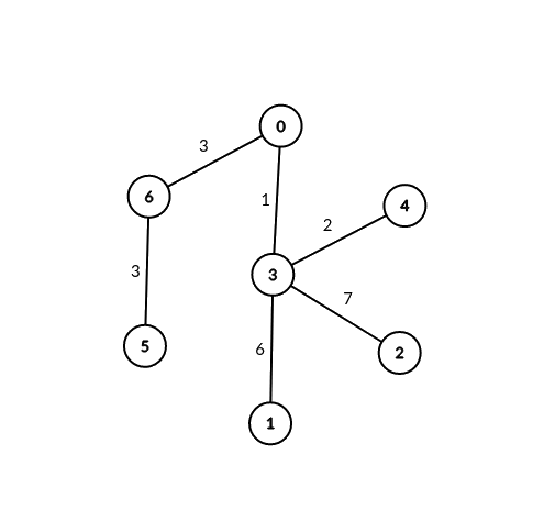
Input: edges = [[0,6,3],[6,5,3],[0,3,1],[3,2,7],[3,1,6],[3,4,2]], signalSpeed = 3
Output: [2,0,0,0,0,0,2]
Explanation: Through server 0, there are 2 pairs of connectable servers: (4, 5) and (4, 6).
Through server 6, there are 2 pairs of connectable servers: (4, 5) and (0, 5).
It can be shown that no two servers are connectable through servers other than 0 and 6.
Constraints:
2 <= n <= 1000edges.length == n - 1edges[i].length == 30 <= ai, bi < nedges[i] = [ai, bi, weighti]1 <= weighti <= 1061 <= signalSpeed <= 106edges represents a valid tree.Problem Overview: You are given a weighted tree representing a network of servers. For every server acting as a signal source, count pairs of other servers whose shortest path distances from that source are divisible by signalSpeed and lie in different branches of the tree. The goal is to compute how many such connectable pairs exist for every node.
Approach 1: DFS with Path Tracking (O(n²) time, O(n) space)
Treat each server as the root of the signal. From that root, run DFS into each neighboring branch and track cumulative path distance. For every visited node, check distance % signalSpeed == 0. Maintain a count of valid nodes discovered in each branch. Since connectable pairs must come from different branches, combine counts using multiplication: if branch A has a valid nodes and branch B has b, they contribute a * b pairs. Repeat this process for every node as the source. The algorithm relies on adjacency lists and recursive traversal of the tree. Time complexity is O(n²) because a DFS runs from each node, while space complexity is O(n) for recursion and distance tracking.
Approach 2: Centroid Decomposition with DFS (O(n log n) time, O(n) space)
Centroid decomposition reduces repeated traversal in large trees. Instead of running full DFS from every node, repeatedly split the tree around a centroid node that balances subtree sizes. For each centroid, run DFS through its subtrees and compute path distances modulo signalSpeed. Track how many nodes satisfy the divisibility condition and merge counts across subtrees to form valid pairs. Because each decomposition level processes disjoint subtrees and the tree height shrinks logarithmically, the overall complexity becomes O(n log n). This method combines depth-first search with divide‑and‑conquer on the tree structure.
Recommended for interviews: The DFS with path tracking approach is usually expected first because it clearly models the branching constraint and shows strong understanding of tree traversal. Once that works, discussing centroid decomposition demonstrates advanced optimization skills and awareness of scalable tree-processing techniques.
| Approach | Time | Space | When to Use |
|---|---|---|---|
| DFS with Path Tracking | O(n²) | O(n) | Best for interviews and moderate constraints where running DFS from each node is acceptable |
| Centroid Decomposition with DFS | O(n log n) | O(n) | Large trees where repeated full traversals are expensive; demonstrates advanced tree optimization |