
Boundary of Binary Tree - Video Solutions
LeetCode 545. Boundary of Binary Tree
Boundary of Binary Tree - Video Solution
Watch 10 video solutions for Boundary of Binary Tree, a medium level problem involving Tree, Depth-First Search, Binary Tree. This walkthrough by Happy Coding has 6,697 views views. Want to try solving it yourself? Practice on FleetCode or read the detailed text solution.
Problem Statement
The boundary of a binary tree is the concatenation of the root, the left boundary, the leaves ordered from left-to-right, and the reverse order of the right boundary.
The left boundary is the set of nodes defined by the following:
- The root node's left child is in the left boundary. If the root does not have a left child, then the left boundary is empty.
- If a node is in the left boundary and has a left child, then the left child is in the left boundary.
- If a node is in the left boundary, has no left child, but has a right child, then the right child is in the left boundary.
- The leftmost leaf is not in the left boundary.
The right boundary is similar to the left boundary, except it is the right side of the root's right subtree. Again, the leaf is not part of the right boundary, and the right boundary is empty if the root does not have a right child.
The leaves are nodes that do not have any children. For this problem, the root is not a leaf.
Given the root of a binary tree, return the values of its boundary.
Example 1:
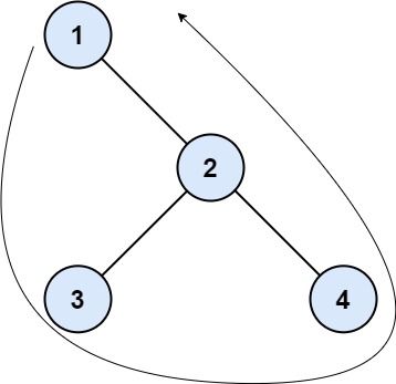
Input: root = [1,null,2,3,4]
Output: [1,3,4,2]
Explanation:
- The left boundary is empty because the root does not have a left child.
- The right boundary follows the path starting from the root's right child 2 -> 4.
  4 is a leaf, so the right boundary is [2].
- The leaves from left to right are [3,4].
Concatenating everything results in [1] + [] + [3,4] + [2] = [1,3,4,2].
Example 2:
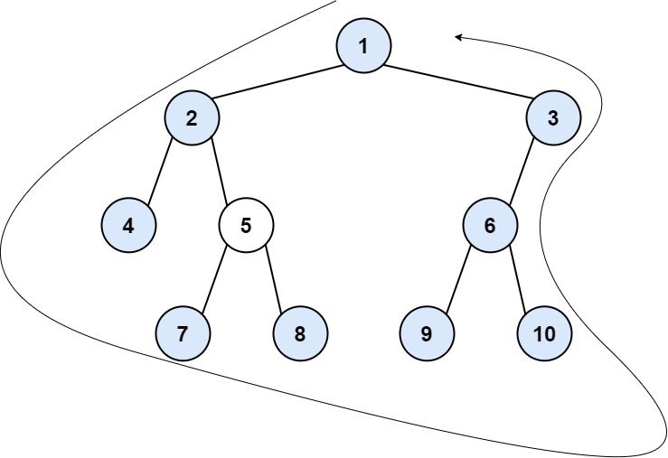
Input: root = [1,2,3,4,5,6,null,null,null,7,8,9,10]
Output: [1,2,4,7,8,9,10,6,3]
Explanation:
- The left boundary follows the path starting from the root's left child 2 -> 4.
  4 is a leaf, so the left boundary is [2].
- The right boundary follows the path starting from the root's right child 3 -> 6 -> 10.
  10 is a leaf, so the right boundary is [3,6], and in reverse order is [6,3].
- The leaves from left to right are [4,7,8,9,10].
Concatenating everything results in [1] + [2] + [4,7,8,9,10] + [6,3] = [1,2,4,7,8,9,10,6,3].
Constraints:
- The number of nodes in the tree is in the range
[1, 104]. -1000 <= Node.val <= 1000
Approach Overview
Problem Overview: Given a binary tree, return its boundary traversal in anti-clockwise order starting from the root. The boundary includes the left boundary, all leaf nodes, and the right boundary (added in reverse order) without duplicates.
Approach 1: DFS with Boundary Classification (O(n) time, O(h) space)
This approach performs a depth-first traversal while classifying each node as part of the left boundary, right boundary, or a leaf. The root is always included first. During DFS, you propagate two flags: isLeftBoundary and isRightBoundary. If a node is on the left boundary, append it before exploring children. If it is a leaf (no children), add it directly. If it is on the right boundary, append it after exploring children so the final order becomes reversed automatically. This technique ensures each node is processed exactly once, giving O(n) time complexity and O(h) recursion stack space where h is tree height. The traversal naturally fits problems involving depth-first search on a binary tree.
Approach 2: Separate Traversals for Left Boundary, Leaves, and Right Boundary (O(n) time, O(h) space)
This method splits the work into three clear steps. First, iterate down the left side of the tree and collect non-leaf nodes to build the left boundary. Second, run a DFS across the tree to collect all leaf nodes in left-to-right order. Third, traverse the right side of the tree and push non-leaf nodes to a temporary list, then reverse it before appending to the result. Each step touches nodes at most once, so the total runtime remains O(n). Space complexity is O(h) due to recursion during the leaf DFS and the temporary storage for the right boundary. The logic is straightforward and commonly used in tree traversal problems.
Recommended for interviews: The DFS boundary-classification approach is usually preferred. It processes the tree in a single traversal and demonstrates strong control over DFS state and traversal order. The three-step traversal approach is easier to reason about and still optimal, which makes it a good starting point during interviews before refining into the single-pass DFS solution.
Complexity Analysis
| Approach | Time | Space | When to Use |
|---|---|---|---|
| DFS with Boundary Classification | O(n) | O(h) | Best general solution. Processes the tree in one traversal while maintaining boundary state. |
| Separate Left Boundary, Leaves, Right Boundary Traversals | O(n) | O(h) | Good when clarity matters. Splits the boundary logic into simple steps. |