
Sum of Matrix After Queries - Solution & Explanation
Problem Statement
You are given an integer n and a 0-indexed 2D array queries where queries[i] = [typei, indexi, vali].
Initially, there is a 0-indexed n x n matrix filled with 0's. For each query, you must apply one of the following changes:
- if
typei == 0, set the values in the row withindexitovali, overwriting any previous values. - if
typei == 1, set the values in the column withindexitovali, overwriting any previous values.
Return the sum of integers in the matrix after all queries are applied.
Example 1:
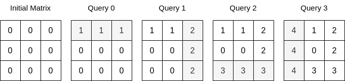
Input: n = 3, queries = [[0,0,1],[1,2,2],[0,2,3],[1,0,4]]
Output: 23
Explanation: The image above describes the matrix after each query. The sum of the matrix after all queries are applied is 23.
Example 2:
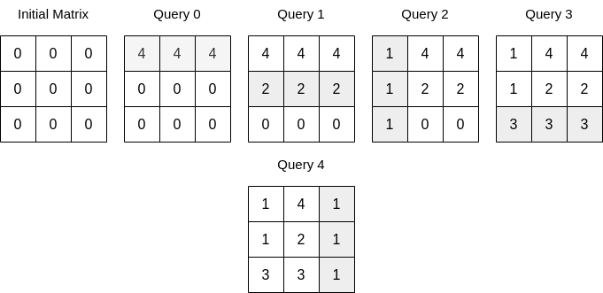
Input: n = 3, queries = [[0,0,4],[0,1,2],[1,0,1],[0,2,3],[1,2,1]]
Output: 17
Explanation: The image above describes the matrix after each query. The sum of the matrix after all queries are applied is 17.
Constraints:
1 <= n <= 1041 <= queries.length <= 5 * 104queries[i].length == 30 <= typei <= 10 <= indexi < n0 <= vali <= 105
Approach Overview
Problem Overview: You start with an n x n matrix filled with zeros. Each query assigns a value to an entire row or column. After processing all queries, return the total sum of the matrix. The challenge is avoiding an expensive full matrix update for every query.
Approach 1: Direct Simulation with Efficient Storage (O(q * n) time, O(n) space)
The straightforward strategy simulates each query as it appears. For a row assignment, iterate across all n columns and update the row values; for a column assignment, iterate through all rows. Instead of storing the entire matrix, you can maintain row and column structures that represent current values and compute contributions to the total sum while applying updates. This reduces memory overhead but still performs O(n) work per query. When the number of queries is small or n is limited, this approach is simple and easy to implement using basic array operations.
Approach 2: Optimized Reverse Simulation (O(q) time, O(n) space)
The key observation: the last assignment to a row or column determines the final value of its cells. Instead of simulating forward, iterate through the queries in reverse. Maintain two hash table or set structures: one for rows already processed and one for columns already processed. When you encounter a row assignment that hasn’t been processed yet, it contributes value * (n - processedCols) to the total because only columns not finalized will keep that value. Mark the row as processed. Similarly, a column assignment contributes value * (n - processedRows). This eliminates repeated overwrites and ensures each row and column is counted at most once.
Reverse simulation works because later queries override earlier ones. By processing from the end, you capture only the assignments that actually survive in the final matrix. The algorithm touches each query once and performs constant-time lookups using sets, which makes it highly scalable even when n and the query count are large.
Recommended for interviews: The reverse simulation approach is what interviewers expect. Writing the direct simulation first shows you understand the mechanics of the problem, but recognizing that only the last assignment matters demonstrates stronger algorithmic insight. Efficient tracking with sets and careful counting of remaining rows or columns leads to the optimal O(q) solution.
Approach 1: Direct Simulation with Efficient Storage
Instead of updating a full matrix, which could be inefficient considering the constraints, we simulate the updates using arrays to keep track of row and column updates. This avoids the need to modify the entire matrix, thus saving computation time and space.
This solution uses two arrays, one for row updates and another for column updates, to store the latest query operation on each row and column. The arrays row_updates and col_updates record the index of the last query that affected each row or column. The computation of the final matrix sum happens by choosing the latest applicable query update for each cell.
Complexity
Time Complexity: O(n^2) - We iterate over all cells to compute the final sum.
Space Complexity: O(n) - We use auxiliary arrays for row and column update indices and values.
Approach 2: Optimized Reverse Simulation
By processing the queries in reverse order, we can efficiently manage the rows and columns to prevent unnecessary overwrites. By using flags to record rows and columns that have already been set, we can avoid redundant operations and achieve an optimized simulation.
This JavaScript solution processes queries in reverse to track which rows and columns have been set. By using boolean arrays to mark applied operations, we accumulate sums only for the first (in reverse order) applicable update, thus minimizing redundant calculations.
Code
JavaScript
C++
Complexity
Time Complexity: O(q + n) - We iterate over queries and use constant space checks.
Space Complexity: O(n) - We use flag arrays for row and column operations.
Approach 3: Hash Table
Since the value of each row and column depends on the last modification, we can traverse all queries in reverse order and use hash tables row and col to record which rows and columns have been modified.
For each query (t, i, v):
- If
t = 0, we check whether theith row has been modified. If not, we addv times (n - |col|)to the answer, where|col|represents the size ofcol, and then additorow. - If
t = 1, we check whether theith column has been modified. If not, we addv times (n - |row|)to the answer, where|row|represents the size ofrow, and then additocol.
Finally, return the answer.
The time complexity is O(m), and the space complexity is O(n). Here, m represents the number of queries.
Code
Python
Java
C++
Go
TypeScript
Complexity Comparison
| Approach | Complexity |
|---|---|
| Direct Simulation with Efficient Storage | Time Complexity: O(n^2) - We iterate over all cells to compute the final sum. |
| Optimized Reverse Simulation | Time Complexity: O(q + n) - We iterate over queries and use constant space checks. |
| Hash Table | — |
Detailed Complexity Analysis
| Approach | Time | Space | When to Use |
|---|---|---|---|
| Direct Simulation with Efficient Storage | O(q * n) | O(n) | When constraints are small or when implementing a quick baseline solution |
| Optimized Reverse Simulation | O(q) | O(n) | Best for large inputs where many queries overwrite previous updates |
Video Solution
Leetcode Weekly contest 348 - Medium - Sum of Matrix After Queries • Prakhar Agrawal • 2,143 views views
Watch 9 more video solutions →Frequently Asked Questions
Is Sum of Matrix After Queries easy or hard?
Sum of Matrix After Queries Python/Java solution
How to solve Sum of Matrix After Queries in O(n)?
What is the best approach for Sum of Matrix After Queries?
Is Sum of Matrix After Queries asked at Google/Amazon/Meta?
What data structure is used in Sum of Matrix After Queries?
What is the time complexity of Sum of Matrix After Queries?
Ready to solve this problem?
Practice Sum of Matrix After Queries with our built-in code editor and test cases.
Practice on FleetCodeProblem Info
Table of Contents
Practice this problem
Open in Editor