
Pacific Atlantic Water Flow - Solution & Explanation
Problem Statement
There is an m x n rectangular island that borders both the Pacific Ocean and Atlantic Ocean. The Pacific Ocean touches the island's left and top edges, and the Atlantic Ocean touches the island's right and bottom edges.
The island is partitioned into a grid of square cells. You are given an m x n integer matrix heights where heights[r][c] represents the height above sea level of the cell at coordinate (r, c).
The island receives a lot of rain, and the rain water can flow to neighboring cells directly north, south, east, and west if the neighboring cell's height is less than or equal to the current cell's height. Water can flow from any cell adjacent to an ocean into the ocean.
Return a 2D list of grid coordinates result where result[i] = [ri, ci] denotes that rain water can flow from cell (ri, ci) to both the Pacific and Atlantic oceans.
Example 1:
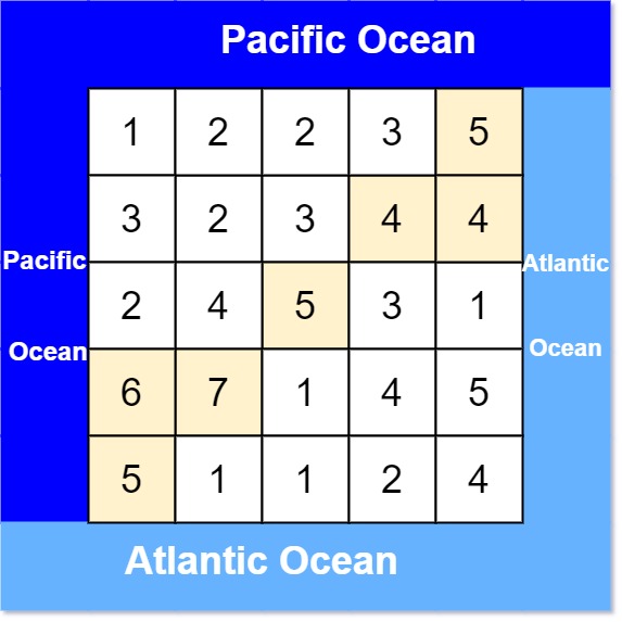
Input: heights = [[1,2,2,3,5],[3,2,3,4,4],[2,4,5,3,1],[6,7,1,4,5],[5,1,1,2,4]]
Output: [[0,4],[1,3],[1,4],[2,2],[3,0],[3,1],[4,0]]
Explanation: The following cells can flow to the Pacific and Atlantic oceans, as shown below:
[0,4]: [0,4] -> Pacific Ocean
       [0,4] -> Atlantic Ocean
[1,3]: [1,3] -> [0,3] -> Pacific Ocean
       [1,3] -> [1,4] -> Atlantic Ocean
[1,4]: [1,4] -> [1,3] -> [0,3] -> Pacific Ocean
       [1,4] -> Atlantic Ocean
[2,2]: [2,2] -> [1,2] -> [0,2] -> Pacific Ocean
       [2,2] -> [2,3] -> [2,4] -> Atlantic Ocean
[3,0]: [3,0] -> Pacific Ocean
       [3,0] -> [4,0] -> Atlantic Ocean
[3,1]: [3,1] -> [3,0] -> Pacific Ocean
       [3,1] -> [4,1] -> Atlantic Ocean
[4,0]: [4,0] -> Pacific Ocean
       [4,0] -> Atlantic Ocean
Note that there are other possible paths for these cells to flow to the Pacific and Atlantic oceans.
Example 2:
Input: heights = [[1]]
Output: [[0,0]]
Explanation: The water can flow from the only cell to the Pacific and Atlantic oceans.
Constraints:
m == heights.lengthn == heights[r].length1 <= m, n <= 2000 <= heights[r][c] <= 105
Approach Overview
Problem Overview: You are given an m x n height matrix where water can flow from a cell to neighboring cells with equal or lower height. The Pacific touches the left and top edges, and the Atlantic touches the right and bottom edges. Return all coordinates where water can flow to both oceans.
Approach 1: Depth-First Search (DFS) from Ocean Borders (O(m*n) time, O(m*n) space)
The key insight is to reverse the thinking. Instead of starting from every cell and checking if water reaches an ocean, start DFS from the ocean borders and move inward. From each ocean edge, run DFS to neighbors with height >= current. This simulates water flowing in reverse. Maintain two visited matrices: one for Pacific reachability and one for Atlantic reachability. After DFS completes, iterate through the grid and collect cells reachable from both. This approach uses recursion and works naturally with grid traversal problems involving depth-first search on a matrix.
Approach 2: Breadth-First Search (BFS) Multi-Source Traversal (O(m*n) time, O(m*n) space)
This approach applies the same reverse-flow insight but replaces recursion with queues. Initialize two BFS queues with all Pacific border cells and Atlantic border cells respectively. Perform BFS while only moving to neighbors with height greater than or equal to the current cell. Track visited cells for each ocean using boolean grids. Once both traversals finish, scan the grid and add coordinates that appear in both visited sets. BFS avoids recursion depth limits and is often preferred when implementing graph traversal on large grids using breadth-first search.
Recommended for interviews: Interviewers expect the reverse traversal idea with DFS or BFS. A brute force approach (checking reachability from every cell) shows initial reasoning but runs in O((m*n)^2). The multi-source DFS/BFS solution reduces it to O(m*n) and demonstrates strong understanding of graph traversal on a grid and how to flip the search direction to avoid redundant work.
Approach 1: Depth-First Search (DFS) Approach
This approach involves performing a DFS from the cells adjacent to the Pacific and Atlantic oceans separately to determine reachable cells for each ocean and then finding their intersection.
The Pacific Ocean can be reached from any cell on the top row or leftmost column. Similarly, the Atlantic Ocean can be reached from any cell on the bottom row or rightmost column. We perform DFS from these boundary cells to mark all cells that can flow into the corresponding ocean. Finally, the intersection of these two sets gives cells that can reach both oceans.
The above function defines a DFS method and applies it from each pacific and atlantic border cell. For pacific, it applies DFS from top row and left column, while for atlantic, it's from bottom row and right column.
DFS explores in four directions, making recursive calls when conditions are satisfied, and keeps track of reachable cells using sets.
Code
Python
Java
C++
JavaScript
C#
Complexity
Time Complexity: O(m * n), where m is the number of rows and n is the number of columns. Each cell is processed once for each ocean.
Space Complexity: O(m * n), as sets used to keep track of visited cells for both oceans.
Approach 2: Breadth-First Search (BFS) Approach
Instead of DFS, we can use BFS to achieve a similar result. This involves starting from the ocean-bordering cells and performing a level-order traversal to mark reachable cells, iteratively checking neighbors in a queue-based manner. BFS might be preferred in scenarios where recursion depth in DFS isn't ideal or could lead to stack overflow.
The idea is to initiate BFS from each ocean's boundary simultaneously, progressively marking each reachable cell, and determining intersecting positions for final results.
This function uses a deque to implement BFS from both Pacific and Atlantic borders. Starting points are defined for each ocean, and a queue processes each cell, enqueuing adjacent cells that retain valid flow conditions.
The results are gathered similarly by intersecting valid Pacific and Atlantic reachable positions.
Complexity
Time Complexity: O(m * n), where BFS is performed from a subset of cells and checks neighbors iteratively.
Space Complexity: O(m * n), contingent upon queue operations and reachability matrices.
Approach 3: BFS
We can start from the boundaries of the Pacific and Atlantic oceans and perform breadth-first search (BFS) respectively to find all cells that can flow to the Pacific and Atlantic oceans. Finally, we take the intersection of the two results, which represents cells that can flow to both the Pacific and Atlantic oceans.
Specifically, we define a queue q_1 to store all cells adjacent to the Pacific ocean, and define a boolean matrix vis_1 to record which cells can flow to the Pacific ocean. Similarly, we define queue q_2 and boolean matrix vis_2 to handle the Atlantic ocean. Initially, we add all cells adjacent to the Pacific ocean to queue q_1 and mark them as visited in vis_1. Similarly, we add all cells adjacent to the Atlantic ocean to queue q_2 and mark them as visited in vis_2.
Then, we perform BFS on q_1 and q_2 respectively. In each BFS, we dequeue a cell (x, y) from the queue and check its four adjacent cells (nx, ny). If an adjacent cell is within the matrix bounds, has not been visited, and its height is not less than the current cell's height (i.e., water can flow to that cell), we add it to the queue and mark it as visited.
Finally, we traverse the entire matrix to find cells that are marked as visited in both vis_1 and vis_2. These cells are our answer.
The time complexity is O(m times n) and the space complexity is O(m times n), where m and n are the number of rows and columns in the matrix, respectively.
Complexity Comparison
| Approach | Complexity |
|---|---|
| Depth-First Search (DFS) Approach | Time Complexity: O(m * n), where m is the number of rows and n is the number of columns. Each cell is processed once for each ocean. Space Complexity: O(m * n), as sets used to keep track of visited cells for both oceans. |
| Breadth-First Search (BFS) Approach | Time Complexity: O(m * n), where BFS is performed from a subset of cells and checks neighbors iteratively. Space Complexity: O(m * n), contingent upon queue operations and reachability matrices. |
| BFS | — |
Detailed Complexity Analysis
| Approach | Time | Space | When to Use |
|---|---|---|---|
| DFS from Ocean Borders | O(m*n) | O(m*n) | Clean recursive solution when stack depth is manageable and DFS is comfortable to implement |
| BFS Multi-Source Traversal | O(m*n) | O(m*n) | Preferred for iterative implementations or when avoiding recursion limits on large grids |
Video Solution
Pacific Atlantic Water Flow - Leetcode 417 - Python • NeetCode • 296,391 views views
Watch 9 more video solutions →Frequently Asked Questions
Is Pacific Atlantic Water Flow easy or hard?
Pacific Atlantic Water Flow Python/Java solution
How to solve Pacific Atlantic Water Flow in O(n)?
What is the best approach for Pacific Atlantic Water Flow?
Is Pacific Atlantic Water Flow asked at Google/Amazon/Meta?
What data structure is used in Pacific Atlantic Water Flow?
What is the time complexity of Pacific Atlantic Water Flow?
Ready to solve this problem?
Practice Pacific Atlantic Water Flow with our built-in code editor and test cases.
Practice on FleetCodeProblem Info
Table of Contents
Practice this problem
Open in Editor