
Modify Graph Edge Weights - Solution & Explanation
Problem Statement
You are given an undirected weighted connected graph containing n nodes labeled from 0 to n - 1, and an integer array edges where edges[i] = [ai, bi, wi] indicates that there is an edge between nodes ai and bi with weight wi.
Some edges have a weight of -1 (wi = -1), while others have a positive weight (wi > 0).
Your task is to modify all edges with a weight of -1 by assigning them positive integer values in the range [1, 2 * 109] so that the shortest distance between the nodes source and destination becomes equal to an integer target. If there are multiple modifications that make the shortest distance between source and destination equal to target, any of them will be considered correct.
Return an array containing all edges (even unmodified ones) in any order if it is possible to make the shortest distance from source to destination equal to target, or an empty array if it's impossible.
Note: You are not allowed to modify the weights of edges with initial positive weights.
Example 1:
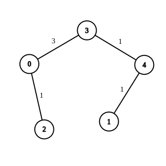
Input: n = 5, edges = [[4,1,-1],[2,0,-1],[0,3,-1],[4,3,-1]], source = 0, destination = 1, target = 5
Output: [[4,1,1],[2,0,1],[0,3,3],[4,3,1]]
Explanation: The graph above shows a possible modification to the edges, making the distance from 0 to 1 equal to 5.
Example 2:
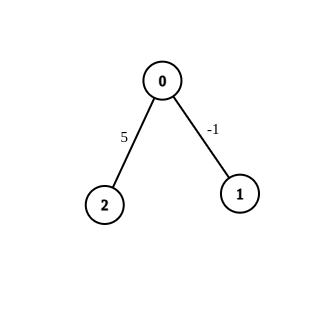
Input: n = 3, edges = [[0,1,-1],[0,2,5]], source = 0, destination = 2, target = 6
Output: []
Explanation: The graph above contains the initial edges. It is not possible to make the distance from 0 to 2 equal to 6 by modifying the edge with weight -1. So, an empty array is returned.
Example 3:
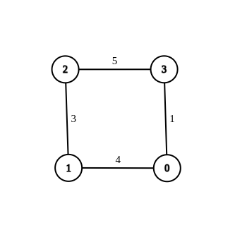
Input: n = 4, edges = [[1,0,4],[1,2,3],[2,3,5],[0,3,-1]], source = 0, destination = 2, target = 6
Output: [[1,0,4],[1,2,3],[2,3,5],[0,3,1]]
Explanation: The graph above shows a modified graph having the shortest distance from 0 to 2 as 6.
Constraints:
1 <= n <= 1001 <= edges.length <= n * (n - 1) / 2edges[i].length == 30 <= ai, bi < nwi = -1or1 <= wi <= 107ai != bi0 <= source, destination < nsource != destination1 <= target <= 109- The graph is connected, and there are no self-loops or repeated edges
Approach Overview
Problem Overview: You are given an undirected graph where some edges have weight -1. Replace those weights with positive values so the shortest path from source to destination equals exactly target. If multiple assignments exist, return any valid graph. If it's impossible, return an empty result.
Approach 1: Dijkstra with Prioritization for -1 Edges (O(m log n) time, O(n + m) space)
This approach treats -1 edges as adjustable during the shortest path computation. Run shortest path using Dijkstra while initially assigning minimal values to unknown edges. When the path distance is smaller than the target, increase weights of selected -1 edges along the candidate path so the final distance matches the target exactly. A priority queue ensures nodes are processed in increasing distance order. The key insight: delay committing final weights until you know which edges affect the optimal path.
Approach 2: Binary Search on Edge Weights with Dijkstra (O(k * m log n) time, O(n + m) space)
Replace each -1 edge with a candidate weight and verify the resulting shortest path using Dijkstra. Instead of guessing blindly, binary search the value range for one adjustable edge while keeping others minimal. Each check runs a shortest path computation on the graph. If the path length becomes larger than the target, reduce the candidate weight; otherwise increase it. This isolates the exact value that makes the path length equal the target.
Approach 3: Dijkstra's Algorithm with Binary Search (O(k * m log n) time, O(n + m) space)
This variant focuses on gradually enabling -1 edges. First run Dijkstra ignoring unknown edges to determine the baseline distance. If it already equals the target, assign very large weights to unused -1 edges. Otherwise, iteratively activate them with small weights and run Dijkstra again. Binary search determines the precise adjustment needed so the shortest path becomes exactly target. This works well when the number of unknown edges is limited.
Approach 4: Iterative Adjustment with BFS (O(k * (n + m)) time, O(n + m) space)
When weights are treated incrementally, you can run repeated BFS-style relaxations while modifying -1 edges. Start by assigning them the smallest allowed value. If the computed path is too short, incrementally increase selected edges until the distance equals the target. This approach avoids heavy priority queue operations but may require multiple passes across the graph. It is easier to implement but less efficient for dense graphs.
Recommended for interviews: Dijkstra with prioritization for -1 edges. It demonstrates strong understanding of weighted graph traversal and dynamic edge adjustment. Brute-force or iterative checks show the core idea, but the optimized Dijkstra-based approach proves you can control shortest-path constraints while maintaining O(m log n) complexity.
Approach 1: Approach 1: Dijkstra's Algorithm with Binary Search
In this approach, we use Dijkstra's algorithm to calculate the shortest path in the graph. The edges with initial weight -1 are considered candidates for modification. We apply binary search to find the appropriate weights for these edges, constraining the path length from source to destination to be equal to the target.
For edges with weight -1, we replace them with a large number initially (greater than the maximum possible path) and refine these weights using binary search to converge on the optimal configuration.
This solution defines a function to apply Dijkstra's algorithm and uses binary search to refine the weights of -1 edges to achieve the target shortest path. The graph is constructed such that each edge weight is initially the binary search mid value when unknown (-1). We update the search bounds based on whether the constructed path is less than, equal to, or greater than the target.
Code
Python
Complexity
Time Complexity: O(E * log(V) * log(W)), where E is the number of edges, V is the number of vertices, and W is the weight range (binary search range).
Space Complexity: O(V + E), mainly for storing the graph structure and distances.
Approach 2: Approach 2: Iterative Adjustment with BFS
This alternative approach leverages an iterative process to adjust edge weights. Starting with a breadth-first search (BFS)-like traversal, we replace unknown weights and check whether the current path meets or exceeds the target. Adjustments are made iteratively until the desired path length is achieved.
This Java solution employs a modified BFS combined with binary search logic to iteratively refine edge weights. The BFS adaptation is used to assess the impact of current estimations on the maximum path length. Adjustments cease when we obtain the desired critical path or exhaust search options.
Code
Java
Complexity
Time Complexity: O(E * V * log(W)), where E is the number of edges, V is the number of vertices, and W is the binary search range for weights.
Space Complexity: O(V + E) for the graph representation and distance tracking.
Approach 3: Binary Search on Edge Weights
In this approach, we use binary search to determine the appropriate weights to assign to edges with initial weight of -1 such that the shortest path from the source to the destination is equal to the target. The idea is to repeatedly apply Dijkstra's algorithm with modified weights until we find the exact configuration which results in the shortest path distance equal to the target.
The solution first sets up a Bellman-Ford function to find the shortest paths from the source node. It then modifies the graph by trying different weights for the edges with initial weight -1 using binary search range [1, 2*10^9]. If the shortest path possible with current weight setup matches the target, the found setup is printed.
Complexity
Time Complexity: O(VE), where V is the number of vertices and E is the number of edges, for each Bellman-Ford run.
Space Complexity: O(V), where V is the number of vertices for storing distances.
Approach 4: Dijkstra with Prioritization for -1 Edges
This approach leverages Dijkstra's algorithm to calculate the shortest path in the graph with a priority queue. We prioritize paths through existing edges first, checking if adjustments can achieve the target path length. It continuously updates the priority to cover edges that were initially marked with -1 with minimal adjustments. The logic attempts to find if a series of replacements can equate the length of the required path to target.
This C solution utilizes Dijkstra's algorithm to find a shortest path and prioritizes updates to edges initially carrying -1 for achieving target distance. It adjusts according to remaining distance discrepancies using a priority queue.
Complexity
Time Complexity: O(V^2), inefficient but functional, typical for unoptimized Dijkstra approaches, adaptive to graph modifications.
Space Complexity: O(V), storing necessary node visitation states and distances.
Approach 5: Shortest Path (Dijkstra's Algorithm)
First, we ignore the edges with a weight of -1 and use Dijkstra's algorithm to find the shortest distance d from source to destination.
-
If
d < target, it means there is a shortest path composed entirely of positive weight edges. No matter how we modify the edges with a weight of-1, we cannot make the shortest distance fromsourcetodestinationequal totarget. Therefore, there is no modification scheme that satisfies the problem, and we can return an empty array. -
If
d = target, it means there is a shortest path composed entirely of positive weight edges, and its length istarget. In this case, we can modify all edges with a weight of-1to the maximum value2 times 10^9. -
If
d > target, we can try to add an edge with a weight of-1to the graph, set the weight of the edge to1, and then use Dijkstra's algorithm again to find the shortest distancedfromsourcetodestination.- If the shortest distance
d leq target, it means that after adding this edge, the shortest path can be shortened, and the shortest path must pass through this edge. Then we only need to change the weight of this edge totarget-d+1to make the shortest path equal totarget. Then we can modify the remaining edges with a weight of-1to the maximum value2 times 10^9. - If the shortest distance
d > target, it means that after adding this edge, the shortest path will not be shortened. Then we greedily keep the weight of this edge as-1and continue to try to add the remaining edges with a weight of-1.
- If the shortest distance
The time complexity is O(n^3), and the space complexity is O(n^2), where n is the number of points in the graph.
Code
Python
Java
C++
Go
TypeScript
Complexity Comparison
| Approach | Complexity |
|---|---|
| Approach 1: Dijkstra's Algorithm with Binary Search | Time Complexity: O(E * log(V) * log(W)), where E is the number of edges, V is the number of vertices, and W is the weight range (binary search range). Space Complexity: O(V + E), mainly for storing the graph structure and distances. |
| Approach 2: Iterative Adjustment with BFS | Time Complexity: O(E * V * log(W)), where E is the number of edges, V is the number of vertices, and W is the binary search range for weights. Space Complexity: O(V + E) for the graph representation and distance tracking. |
| Binary Search on Edge Weights | Time Complexity: O(VE), where V is the number of vertices and E is the number of edges, for each Bellman-Ford run. |
| Dijkstra with Prioritization for -1 Edges | Time Complexity: O(V^2), inefficient but functional, typical for unoptimized Dijkstra approaches, adaptive to graph modifications. |
| Shortest Path (Dijkstra's Algorithm) | — |
Detailed Complexity Analysis
| Approach | Time | Space | When to Use |
|---|---|---|---|
| Dijkstra with Prioritization for -1 Edges | O(m log n) | O(n + m) | Best general solution when graph is large and multiple unknown edges exist |
| Binary Search on Edge Weights + Dijkstra | O(k * m log n) | O(n + m) | Useful when searching the correct value for a specific adjustable edge |
| Dijkstra with Binary Search Strategy | O(k * m log n) | O(n + m) | When baseline shortest path must be measured before enabling -1 edges |
| Iterative Adjustment with BFS | O(k * (n + m)) | O(n + m) | Simpler implementation when graph size is moderate and weights are adjusted gradually |
Video Solution
Modify Graph Edge Weights | Using Dijkstra | Thought Process | Leetcode 2699 | codestorywithMIK • codestorywithMIK • 12,513 views views
Watch 9 more video solutions →Frequently Asked Questions
Is Modify Graph Edge Weights easy or hard?
How to solve Modify Graph Edge Weights in O(m log n)?
What is the best approach for Modify Graph Edge Weights?
What data structure is used in Modify Graph Edge Weights?
What is the time complexity of Modify Graph Edge Weights?
Is Modify Graph Edge Weights asked at Google, Amazon, or Meta?
Is there a Python or Java solution for Modify Graph Edge Weights?
Ready to solve this problem?
Practice Modify Graph Edge Weights with our built-in code editor and test cases.
Practice on FleetCode