You are given a m x n matrix grid consisting of non-negative integers where grid[row][col] represents the minimum time required to be able to visit the cell (row, col), which means you can visit the cell (row, col) only when the time you visit it is greater than or equal to grid[row][col].
You are standing in the top-left cell of the matrix in the 0th second, and you must move to any adjacent cell in the four directions: up, down, left, and right. Each move you make takes 1 second.
Return the minimum time required in which you can visit the bottom-right cell of the matrix. If you cannot visit the bottom-right cell, then return -1.
Example 1:
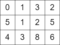
Input: grid = [[0,1,3,2],[5,1,2,5],[4,3,8,6]]
Output: 7
Explanation: One of the paths that we can take is the following:
- at t = 0, we are on the cell (0,0).
- at t = 1, we move to the cell (0,1). It is possible because grid[0][1] <= 1.
- at t = 2, we move to the cell (1,1). It is possible because grid[1][1] <= 2.
- at t = 3, we move to the cell (1,2). It is possible because grid[1][2] <= 3.
- at t = 4, we move to the cell (1,1). It is possible because grid[1][1] <= 4.
- at t = 5, we move to the cell (1,2). It is possible because grid[1][2] <= 5.
- at t = 6, we move to the cell (1,3). It is possible because grid[1][3] <= 6.
- at t = 7, we move to the cell (2,3). It is possible because grid[2][3] <= 7.
The final time is 7. It can be shown that it is the minimum time possible.
Example 2:
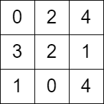
Input: grid = [[0,2,4],[3,2,1],[1,0,4]]
Output: -1
Explanation: There is no path from the top left to the bottom-right cell.
Constraints:
m == grid.lengthn == grid[i].length2 <= m, n <= 10004 <= m * n <= 1050 <= grid[i][j] <= 105grid[0][0] == 0
Problem Overview: You are given a grid where grid[i][j] represents the earliest time you can enter that cell. Starting at the top-left cell, you move in four directions and each move costs one second. The goal is to reach the bottom-right cell in the minimum possible time while respecting each cell's time constraint.
Approach 1: Priority Queue with Dijkstra-Like Approach (O(mn log(mn)))
This problem behaves like a shortest path search on a weighted grid. Treat every cell as a node and each movement as an edge with cost 1, but you may need to wait before entering a cell if its allowed time hasn't been reached. Use a min-heap (priority queue) to always expand the position with the smallest current time, similar to Dijkstra’s algorithm. When exploring a neighbor, compute the earliest time you can step into it; if your arrival time is earlier than grid[r][c], you must wait, and parity adjustments may be required to ensure movement timing works with alternating steps.
The priority queue ensures cells are processed in increasing time order, guaranteeing the first time you reach the destination is optimal. Maintain a visited or distance matrix to avoid redundant processing. Time complexity is O(mn log(mn)) because each cell may be pushed into the heap and heap operations cost logarithmic time. Space complexity is O(mn) for the heap and distance tracking. This technique is a classic application of graph shortest path combined with a priority queue on a matrix.
Approach 2: Breadth-First Search with Level Traversal (O(mn))
A modified BFS can also traverse the grid while tracking time levels. Instead of simple layer expansion, you compute the earliest valid time to enter each neighbor and adjust the traversal level accordingly. If the neighbor's required time is larger than your next step, you simulate waiting by increasing the effective time until the move becomes valid. This sometimes introduces parity adjustments similar to the Dijkstra solution.
BFS works because all moves have uniform cost, but managing waiting times and revisiting states makes the implementation trickier. A queue processes states in increasing time order while storing the earliest reachable time for each cell. With proper pruning, each cell is processed only a limited number of times. Time complexity is approximately O(mn) with O(mn) space for the queue and visitation tracking. This approach emphasizes traversal mechanics from Breadth-First Search but requires careful time calculations.
Recommended for interviews: The Dijkstra-style priority queue approach is what most interviewers expect. The grid naturally forms a weighted graph where arrival time matters, making a min-heap the most intuitive and reliable solution. Mentioning BFS first shows you recognize the grid traversal pattern, but switching to a heap-based shortest path demonstrates stronger algorithmic judgment.
This approach uses a priority queue to implement a modified version of Dijkstra's algorithm. The challenge here includes managing both the time constraints specified by the grid and the movement cost. The goal is to find the shortest path in terms of time while making sure each cell is entered at a valid time.
We use a priority queue to determine which cell to visit next based on the minimum time it takes to safely visit it. This is similar to choosing the shortest weighted edge in Dijkstra's algorithm, but our 'weight' here is the time passed.
The Python solution uses a heap priority queue to manage cells to visit by their prospective visit time. We maintain a set of visited cells to prevent re-evaluation. For each cell, we consider its neighboring cells and calculate any necessary wait time based on the grid's constraints.
Python
Java
C++
JavaScript
Time Complexity: O(m*n*log(m*n)) due to heap operations for each cell.
Space Complexity: O(m*n) to store the visited set.
This approach uses a breadth-first search (BFS) where we evaluate the grid level by level. Instead of using a priority queue, the BFS explores nodes in increasing order of time levels, trying to meet grid constraints at each level. It tracks the earliest time a cell can be safely visited.
The Python solution applies BFS using a deque structure to simulate levels of operation, maintaining an auxiliary matrix to record the earliest times a cell can be visited, ensuring grid constraints are respected.
Python
Java
C++
JavaScript
Time Complexity: O(m*n)
Space Complexity: O(m*n)
We observe that if we cannot move at the cell (0, 0), i.e., grid[0][1] > 1 and grid[1][0] > 1, then we cannot move at the cell (0, 0) anymore, and we should return -1. For other cases, we can move.
Next, we define dist[i][j] to represent the earliest arrival time at (i, j). Initially, dist[0][0] = 0, and the dist of other positions are all initialized to infty.
We use a priority queue (min heap) to maintain the cells that can currently move. The elements in the priority queue are (dist[i][j], i, j), i.e., (dist[i][j], i, j) represents the earliest arrival time at (i, j).
Each time we take out the cell (t, i, j) that can arrive the earliest from the priority queue. If (i, j) is (m - 1, n - 1), then we directly return t. Otherwise, we traverse the four adjacent cells (x, y) of (i, j), which are up, down, left, and right. If t + 1 < grid[x][y], then the time nt = grid[x][y] + (grid[x][y] - (t + 1)) bmod 2 to move to (x, y). At this time, we can repeatedly move to extend the time to no less than grid[x][y], depending on the parity of the distance between t + 1 and grid[x][y]. Otherwise, the time nt = t + 1 to move to (x, y). If nt < dist[x][y], then we update dist[x][y] = nt, and add (nt, x, y) to the priority queue.
The time complexity is O(m times n times log (m times n)), and the space complexity is O(m times n). Where m and n are the number of rows and columns of the grid, respectively.
Python
Java
C++
Go
TypeScript
JavaScript
| Approach | Complexity |
|---|---|
| Priority Queue with Dijkstra-Like Approach | Time Complexity: O(m*n*log(m*n)) due to heap operations for each cell. |
| Breadth-First Search with Level Traversal | Time Complexity: O(m*n) |
| Shortest Path + Priority Queue (Min Heap) | — |
| Approach | Time | Space | When to Use |
|---|---|---|---|
| Priority Queue with Dijkstra-Like Approach | O(mn log(mn)) | O(mn) | Best general solution for shortest path with time constraints. Reliable and commonly expected in interviews. |
| Breadth-First Search with Level Traversal | O(mn) | O(mn) | Useful when modeling traversal levels directly and handling wait times carefully. |
Minimum Time to Visit a Cell In a Grid - Leetcode 2577 - Python • NeetCodeIO • 12,047 views views
Watch 9 more video solutions →Practice Minimum Time to Visit a Cell In a Grid with our built-in code editor and test cases.
Practice on FleetCode