You are given a 0-indexed 2D integer array grid of size m x n. Each cell has one of two values:
0 represents an empty cell,1 represents an obstacle that may be removed.You can move up, down, left, or right from and to an empty cell.
Return the minimum number of obstacles to remove so you can move from the upper left corner (0, 0) to the lower right corner (m - 1, n - 1).
Example 1:
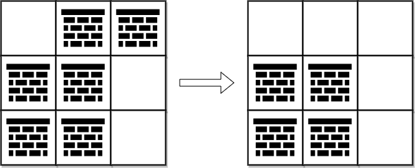
Input: grid = [[0,1,1],[1,1,0],[1,1,0]]
Output: 2
Explanation: We can remove the obstacles at (0, 1) and (0, 2) to create a path from (0, 0) to (2, 2).
It can be shown that we need to remove at least 2 obstacles, so we return 2.
Note that there may be other ways to remove 2 obstacles to create a path.
Example 2:
Input: grid = [[0,1,0,0,0],[0,1,0,1,0],[0,0,0,1,0]]
Output: 0
Explanation: We can move from (0, 0) to (2, 4) without removing any obstacles, so we return 0.
Constraints:
m == grid.lengthn == grid[i].length1 <= m, n <= 1052 <= m * n <= 105grid[i][j] is either 0 or 1.grid[0][0] == grid[m - 1][n - 1] == 0Problem Overview: You start at the top-left cell of a binary grid and want to reach the bottom-right corner. Cells with 0 are free, while 1 represents an obstacle that must be removed before entering. The goal is to reach the destination while removing the minimum number of obstacles.
Approach 1: Dijkstra-like Algorithm (O(m*n log(m*n)) time, O(m*n) space)
This grid can be modeled as a weighted graph where each cell is a node. Moving into a free cell has cost 0, and moving into an obstacle has cost 1 because you must remove it. Use a priority queue to always expand the cell with the smallest accumulated obstacle removals. Maintain a distance matrix storing the minimum removals required to reach each cell. Each step explores the four directions and updates the cost using the classic relaxation step from shortest path algorithms.
The priority queue ensures the smallest removal count is processed first, exactly like Dijkstra’s algorithm on a weighted graph. This approach works reliably for any grid and is easy to reason about during interviews. Complexity is O(m*n log(m*n)) due to heap operations, and space is O(m*n) for the distance matrix and queue.
Approach 2: Dynamic Programming with Monotonic Queue (0-1 BFS) (O(m*n) time, O(m*n) space)
The key observation is that edge weights are only 0 or 1. That allows replacing the heap with a deque using the 0-1 BFS technique. When moving to a free cell (0), push the position to the front of the deque. When moving into an obstacle (1), push it to the back. This ordering guarantees cells with fewer removals are processed first without a priority queue.
You still maintain a distance matrix to avoid revisiting cells with a worse cost. Each cell is processed at most once per optimal distance update, so the total complexity becomes linear in the grid size: O(m*n). This method is a specialized optimization of Breadth-First Search for weighted edges with values 0 or 1 and is common in grid-based graph problems.
Recommended for interviews: Start by explaining the graph interpretation and the Dijkstra-style solution. Interviewers expect candidates to recognize the shortest path formulation. Then point out that weights are only 0 or 1, which enables the optimized 0-1 BFS with a deque. Demonstrating both approaches shows strong understanding of graph algorithms and practical optimization techniques.
This approach uses a priority queue (or deque) to implement a modified Dijkstra's algorithm to explore the grid in a way similar to the 0-1 BFS (Breadth-First Search). Here, obstacles count as 'cost', and we try to find the minimum 'cost' path from the top-left corner to the bottom-right corner. We assign a priority based on the number of obstacles removed.
The function initiates a deque with the starting point (0, 0). We use a distance array to store the minimum number of obstacles needed to reach each cell. Using directions for the four possible moves, we attempt moving to adjacent cells, leveraging the property of a deque to prioritize uncosted moves (moves to a 0) via appendleft. In contrast, costly moves (moves to a 1) are added normally with append. The algorithm continues until the target cell is reached with the minimum obstacle count possible.
Time Complexity: O(m * n)
Space Complexity: O(m * n)
In this approach, we utilize dynamic programming combined with a monotonic queue to solve the problem of reaching the bottom-right corner with minimal obstacle removal. This alternative method involves leveraging the properties of dynamic arrays to store and update minimal removal costs dynamically while using a queue to maintain an effective processing order based on current state values.
This dynamic programming version utilizes a monotonic queue to keep the process smooth, in essence maintaining timeline-line transitions amidst evolved states. Adjustments are made based on evaluated costs for obstacles, ensuring ultimately reaching the target state with minimal burdensome path choices.
Time Complexity: O(m * n)
Space Complexity: O(m * n)
This problem is essentially a shortest path model, but we need to find the minimum number of obstacles to remove.
In an undirected graph with edge weights of only 0 and 1, we can use a double-ended queue to perform BFS. The principle is that if the weight of the current point that can be expanded is 0, it is added to the front of the queue; if the weight is 1, it is added to the back of the queue.
If the weight of an edge is
0, then the newly expanded node has the same weight as the current front node, and it can obviously be used as the starting point for the next expansion.
The time complexity is O(m times n), and the space complexity is O(m times n). Where m and n are the number of rows and columns of the grid, respectively.
Similar problems:
Python
Java
C++
Go
TypeScript
| Approach | Complexity |
|---|---|
| Approach 1: Dijkstra-like Algorithm | Time Complexity: O(m * n) |
| Approach 2: Dynamic Programming with Monotonic Queue | Time Complexity: O(m * n) |
| Double-Ended Queue BFS | — |
| Approach | Time | Space | When to Use |
|---|---|---|---|
| Dijkstra-like Algorithm (Priority Queue) | O(m*n log(m*n)) | O(m*n) | General weighted grid problems where edge costs vary and a heap-based shortest path is straightforward. |
| Dynamic Programming with Monotonic Queue (0-1 BFS) | O(m*n) | O(m*n) | Best when edge weights are only 0 or 1, enabling deque-based BFS instead of a priority queue. |
Minimum Obstacle Removal to Reach Corner - Leetcode 2290 - Python • NeetCodeIO • 8,526 views views
Watch 9 more video solutions →Practice Minimum Obstacle Removal to Reach Corner with our built-in code editor and test cases.
Practice on FleetCode