You are given a 0-indexed m x n integer matrix grid. Your initial position is at the top-left cell (0, 0).
Starting from the cell (i, j), you can move to one of the following cells:
(i, k) with j < k <= grid[i][j] + j (rightward movement), or(k, j) with i < k <= grid[i][j] + i (downward movement).Return the minimum number of cells you need to visit to reach the bottom-right cell (m - 1, n - 1). If there is no valid path, return -1.
Example 1:
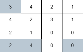
Input: grid = [[3,4,2,1],[4,2,3,1],[2,1,0,0],[2,4,0,0]]
Output: 4
Explanation: The image above shows one of the paths that visits exactly 4 cells.
Example 2:
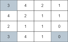
Input: grid = [[3,4,2,1],[4,2,1,1],[2,1,1,0],[3,4,1,0]]
Output: 3
Explanation: The image above shows one of the paths that visits exactly 3 cells.
Example 3:
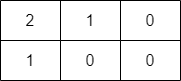
Input: grid = [[2,1,0],[1,0,0]]
Output: -1
Explanation: It can be proven that no path exists.
Constraints:
m == grid.lengthn == grid[i].length1 <= m, n <= 1051 <= m * n <= 1050 <= grid[i][j] < m * ngrid[m - 1][n - 1] == 0Problem Overview: You start at (0,0) in a grid where each cell value tells you how far you can move right or down. From cell (i,j), you can jump to any cell in the same row up to j + grid[i][j] or in the same column up to i + grid[i][j]. The task is to reach (m-1,n-1) while visiting the minimum number of cells.
Approach 1: Breadth-First Search with Row/Column Pruning (O(mn log(m+n)) time, O(mn) space)
This approach models the grid as a graph and performs Breadth-First Search from (0,0). Each step explores all reachable cells in the same row and column within the allowed jump range. A naive BFS would repeatedly scan the same row or column segments, leading to quadratic work. To avoid this, maintain ordered sets (or heaps) of unvisited indices for each row and column. When you process a cell, remove visited indices and only push valid new cells into the queue. Each cell enters the queue once, while set operations add a log factor. This guarantees that BFS levels correspond to the number of visited cells, giving the shortest path automatically.
Approach 2: Dynamic Programming with Greedy Optimization (O(mn log n) time, O(mn) space)
This method combines Dynamic Programming with greedy range queries using heaps (priority queues). Let dp[i][j] represent the minimum visited cells needed to reach (i,j). While scanning the grid row by row, maintain heaps for each row and column storing candidate cells that can reach the current position. Each heap keeps entries ordered by the best dp value. Before using a heap entry, discard it if its reachable range no longer covers the current index. The smallest valid entry gives the optimal predecessor. After computing dp[i][j], push it into the row and column heaps with its maximum reachable boundary. This avoids checking every previous cell and effectively performs greedy minimum selection within valid jump ranges.
The optimization works because each cell contributes to future transitions only within a limited interval, and heaps quickly discard outdated candidates. The idea resembles interval DP combined with monotonic pruning patterns often seen with monotonic structures.
Recommended for interviews: The BFS formulation is the most intuitive because it directly models the problem as shortest path in a grid graph. However, interviewers usually expect the optimized version that avoids scanning entire rows and columns. Showing the naive BFS first demonstrates understanding, while implementing the pruned BFS or the heap-based DP shows strong algorithmic optimization skills.
This approach considers the problem of moving through the grid as a traversal problem where each cell is a node in a graph. We can use a Breadth-First Search (BFS) strategy to explore the shortest path to the target cell. BFS is appropriate as it explores nodes layer by layer and guarantees the shortest path in an unweighted grid like this.
Starting from the top-left cell, we check all possible jumps to cells on the right and below based on the current cell's value and keep track of visited nodes to prevent cycles. When we reach the bottom-right cell, we can return the count of cells visited. If we exhaust all options without reaching the end, we return -1.
The Python solution uses a queue to perform BFS. We start at (0, 0), add it to the queue, and mark it visited. For each cell, explore possible right and down moves, adding them to the queue if they are valid and not visited. We increase the count of steps with each layer of nodes processed in the queue.
Time Complexity: O(m * n) due to potentially exploring each cell once.
Space Complexity: O(m * n) due to storing nodes in the queue and visited set.
In this approach, we apply a dynamic programming strategy with greedy choices to reduce exploration. We maintain a DP table to store the minimum cells visited to reach each point in the grid. At each point, only consider the farthest reachable cells to reduce redundant paths, thereby optimizing the space from the BFS approach.
Carefully choose the most promising moves that optimize the reach towards the target, using current state information to prune paths not beneficial to reaching the destination with fewer steps.
This Python solution uses a deque for dynamic programming iteration to fill a DP table with minimum steps required. Each cell is updated only if a shorter path is found, and only those cells are processed further.
Time Complexity: O(m * n), potential checking every cell.
Space Complexity: O(m * n), storing DP table.
Let's denote the number of rows of the grid as m and the number of columns as n. Define dist[i][j] to be the shortest distance from the coordinate (0, 0) to the coordinate (i, j). Initially, dist[0][0]=1 and dist[i][j]=-1 for all other i and j.
For each grid (i, j), it can come from the grid above or the grid on the left. If it comes from the grid above (i', j), where 0 leq i' \lt i, then (i', j) must satisfy grid[i'][j] + i' geq i. We need to select from these grids the one that is closest.
Therefore, we maintain a priority queue (min-heap) for each column j. Each element of the priority queue is a pair (dist[i][j], i), which represents that the shortest distance from the coordinate (0, 0) to the coordinate (i, j) is dist[i][j]. When we consider the coordinate (i, j), we only need to take out the head element (dist[i'][j], i') of the priority queue. If grid[i'][j] + i' geq i, we can move from the coordinate (i', j) to the coordinate (i, j). At this time, we can update the value of dist[i][j], that is, dist[i][j] = dist[i'][j] + 1, and add (dist[i][j], i) to the priority queue.
Similarly, we can maintain a priority queue for each row i and perform a similar operation.
Finally, we can obtain the shortest distance from the coordinate (0, 0) to the coordinate (m - 1, n - 1), that is, dist[m - 1][n - 1], which is the answer.
The time complexity is O(m times n times log (m times n)) and the space complexity is O(m times n). Here, m and n are the number of rows and columns of the grid, respectively.
| Approach | Complexity |
|---|---|
| Breadth-First Search (BFS) | Time Complexity: O(m * n) due to potentially exploring each cell once. |
| Dynamic Programming with Greedy Optimization | Time Complexity: O(m * n), potential checking every cell. |
| Priority Queue | — |
| Approach | Time | Space | When to Use |
|---|---|---|---|
| Naive BFS scanning rows and columns | O(mn(m+n)) | O(mn) | Conceptual baseline to understand reachable cells |
| BFS with ordered sets / pruning | O(mn log(m+n)) | O(mn) | Efficient shortest-path solution when modeling the grid as a graph |
| Dynamic Programming with heap optimization | O(mn log n) | O(mn) | Best when implementing interval DP with fast minimum queries |
Minimum Number of Visited Cells in a Grid | 2617 | Weekly Contest 340 • codingMohan • 1,764 views views
Watch 6 more video solutions →Practice Minimum Number of Visited Cells in a Grid with our built-in code editor and test cases.
Practice on FleetCode