
Minimum Edge Weight Equilibrium Queries in a Tree - Solution & Explanation
Problem Statement
There is an undirected tree with n nodes labeled from 0 to n - 1. You are given the integer n and a 2D integer array edges of length n - 1, where edges[i] = [ui, vi, wi] indicates that there is an edge between nodes ui and vi with weight wi in the tree.
You are also given a 2D integer array queries of length m, where queries[i] = [ai, bi]. For each query, find the minimum number of operations required to make the weight of every edge on the path from ai to bi equal. In one operation, you can choose any edge of the tree and change its weight to any value.
Note that:
- Queries are independent of each other, meaning that the tree returns to its initial state on each new query.
- The path from
aitobiis a sequence of distinct nodes starting with nodeaiand ending with nodebisuch that every two adjacent nodes in the sequence share an edge in the tree.
Return an array answer of length m where answer[i] is the answer to the ith query.
Example 1:
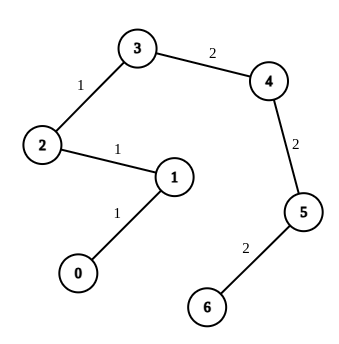
Input: n = 7, edges = [[0,1,1],[1,2,1],[2,3,1],[3,4,2],[4,5,2],[5,6,2]], queries = [[0,3],[3,6],[2,6],[0,6]]
Output: [0,0,1,3]
Explanation: In the first query, all the edges in the path from 0 to 3 have a weight of 1. Hence, the answer is 0.
In the second query, all the edges in the path from 3 to 6 have a weight of 2. Hence, the answer is 0.
In the third query, we change the weight of edge [2,3] to 2. After this operation, all the edges in the path from 2 to 6 have a weight of 2. Hence, the answer is 1.
In the fourth query, we change the weights of edges [0,1], [1,2] and [2,3] to 2. After these operations, all the edges in the path from 0 to 6 have a weight of 2. Hence, the answer is 3.
For each queries[i], it can be shown that answer[i] is the minimum number of operations needed to equalize all the edge weights in the path from ai to bi.
Example 2:
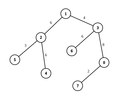
Input: n = 8, edges = [[1,2,6],[1,3,4],[2,4,6],[2,5,3],[3,6,6],[3,0,8],[7,0,2]], queries = [[4,6],[0,4],[6,5],[7,4]]
Output: [1,2,2,3]
Explanation: In the first query, we change the weight of edge [1,3] to 6. After this operation, all the edges in the path from 4 to 6 have a weight of 6. Hence, the answer is 1.
In the second query, we change the weight of edges [0,3] and [3,1] to 6. After these operations, all the edges in the path from 0 to 4 have a weight of 6. Hence, the answer is 2.
In the third query, we change the weight of edges [1,3] and [5,2] to 6. After these operations, all the edges in the path from 6 to 5 have a weight of 6. Hence, the answer is 2.
In the fourth query, we change the weights of edges [0,7], [0,3] and [1,3] to 6. After these operations, all the edges in the path from 7 to 4 have a weight of 6. Hence, the answer is 3.
For each queries[i], it can be shown that answer[i] is the minimum number of operations needed to equalize all the edge weights in the path from ai to bi.
Constraints:
1 <= n <= 104edges.length == n - 1edges[i].length == 30 <= ui, vi < n1 <= wi <= 26- The input is generated such that
edgesrepresents a valid tree. 1 <= queries.length == m <= 2 * 104queries[i].length == 20 <= ai, bi < n
Approach Overview
Problem Overview: You are given a weighted tree and multiple queries. Each query asks for the minimum number of edge weight changes required so that all edges along the path between two nodes have the same weight. The key observation is that the optimal strategy keeps the most frequent weight on that path and changes the rest.
Approach 1: DFS for Path Finding and Frequency Analysis (O(q * n) time, O(n) space)
For each query, run a DFS or BFS to find the path between the two nodes. While traversing, maintain a frequency counter of the edge weights encountered. After reaching the destination, compute the path length and subtract the highest frequency weight on that path. That difference equals the number of operations required. This approach directly simulates the query but recomputes paths repeatedly, which becomes expensive when the number of queries is large.
Approach 2: LCA with Prefix Weight Frequencies (O((n + q) log n) time, O(n * W) space)
Preprocess the tree using a depth-first traversal and compute binary lifting tables for LCA queries. During the DFS, maintain prefix frequency counts for each possible edge weight from the root to every node. For a query (u, v), compute their LCA. The frequency of each weight on the path is derived from prefix arrays: freq[u] + freq[v] - 2 * freq[lca]. The path length is known from node depths, and the minimum operations equal pathLength - maxWeightFrequency. This avoids recomputing paths and makes each query efficient.
This method combines classic tree traversal with graph preprocessing and prefix counting stored in arrays. The core improvement comes from converting repeated path exploration into constant-time frequency reconstruction after an LCA lookup.
Recommended for interviews: Start with the DFS path approach to show you understand the problem and the key observation about keeping the most frequent weight. Then move to the LCA + prefix frequency technique. Interviewers expect this optimization because it reduces repeated work across queries and demonstrates strong understanding of tree preprocessing and query optimization.
Approach 1: DFS for Path Finding and Frequency Analysis
To solve the problem, you can perform a Depth First Search (DFS) or Breadth First Search (BFS) to find the path between each pair of nodes specified in the queries. Once you have the path, count the frequency of each edge weight. The minimum number of operations needed is determined by reducing other weights to the most frequent weight found in the path.
This Python solution constructs the tree from the given edge list using an adjacency list. It then recursively uses DFS to locate paths between the queried nodes. After locating the path, we count the frequency of each edge weight on the path. To find the minimum operation count, we compute the difference between the path length and the frequency of the most common edge weight.
Code
Python
JavaScript
Complexity
Time Complexity: O(n + q *E), where n is the number of nodes, q is the number of queries, and E is the number of edges along the longest path in the tree. This follows because we have to perform a DFS from path a to b for each query.
Space Complexity: O(n + q * E), as we have to store the adjacency list and each path.
Approach 2: LCA for Efficient Path Finding
The Lowest Common Ancestor (LCA) technique helps efficiently identify paths in a tree. Using binary lifting or similar methods, you can determine the path from one node to another with pre-computed parent and depth arrays. This makes querying more efficient, especially in large trees.
This C++ solution implements an efficient path finding through the tree leveraging the Lowest Common Ancestor (LCA) technique. It builds the tree then traverses it to pre-compute parent and depth information. With dynamic programming, it can quickly find paths from queries and analyze weights on these paths, resulting in a time-effective solution.
Complexity
Time Complexity: O(n log n + q log n) due to preprocessing for LCA and sparse table lookups.
Space Complexity: O(n log n), primarily used for LCA preprocessing and storing frequency data.
Approach 3: Binary Lifting for LCA
The problem asks for the minimum number of operations to make all edge weights the same on the path between any two points. This is essentially the length of the path between these two points, minus the number of times the most frequently occurring edge appears on the path.
The length of the path between two points can be obtained by finding the LCA (Lowest Common Ancestor) using binary lifting. Let's denote the two points as u and v, and their LCA as x. Then, the path length from u to v is depth(u) + depth(v) - 2 times depth(x).
Additionally, we can use an array cnt[n][26] to record the number of occurrences of each edge weight from the root node to each node. Then, the number of times the most frequently occurring edge appears on the path from u to v is max_{0 leq j < 26} cnt[u][j] + cnt[v][j] - 2 times cnt[x][j], where x is the LCA of u and v.
The process of finding the LCA using binary lifting is as follows:
We denote the depth of each node as depth, its parent node as p, and f[i][j] as the 2^jth ancestor of node i. Then, for any two points x and y, we can find their LCA as follows:
- If
depth(x) < depth(y), then swapxandy, i.e., ensure that the depth ofxis not less than the depth ofy; - Next, we continuously raise the depth of
xuntil the depths ofxandyare the same, at which point the depths ofxandyare bothdepth(x); - Then, we raise the depths of
xandysimultaneously until the parents ofxandyare the same, at which point the parents ofxandyare bothf[x][0], which is the LCA ofxandy.
Finally, the minimum number of operations from node u to node v is depth(u) + depth(v) - 2 times depth(x) - max_{0 leq j < 26} cnt[u][j] + cnt[v][j] - 2 times cnt[x][j].
The time complexity is O((n + q) times C times log n), and the space complexity is O(n times C times log n). Here, C is the maximum value of the edge weight.
Complexity Comparison
| Approach | Complexity |
|---|---|
| DFS for Path Finding and Frequency Analysis | Time Complexity: O(n + q *E), where n is the number of nodes, q is the number of queries, and E is the number of edges along the longest path in the tree. This follows because we have to perform a DFS from path a to b for each query. Space Complexity: O(n + q * E), as we have to store the adjacency list and each path. |
| LCA for Efficient Path Finding | Time Complexity: O(n log n + q log n) due to preprocessing for LCA and sparse table lookups. Space Complexity: O(n log n), primarily used for LCA preprocessing and storing frequency data. |
| Binary Lifting for LCA | — |
Detailed Complexity Analysis
| Approach | Time | Space | When to Use |
|---|---|---|---|
| DFS Path Search with Frequency Counting | O(q * n) | O(n) | Small trees or very few queries where recomputing paths is acceptable |
| LCA with Prefix Weight Frequencies | O((n + q) log n) | O(n * W) | Large trees and many queries; optimal approach for competitive programming and interviews |
Video Solution
2846. Minimum Edge Weight Equilibrium Queries in a Tree | Binary Lifting | Weekly Leetcode 361 • codingMohan • 2,478 views views
Watch 6 more video solutions →Frequently Asked Questions
Is Minimum Edge Weight Equilibrium Queries in a Tree easy or hard?
Minimum Edge Weight Equilibrium Queries in a Tree Python/Java solution
How to solve Minimum Edge Weight Equilibrium Queries in a Tree in O(n)?
What is the best approach for Minimum Edge Weight Equilibrium Queries in a Tree?
Is Minimum Edge Weight Equilibrium Queries in a Tree asked at Google/Amazon/Meta?
What data structure is used in Minimum Edge Weight Equilibrium Queries in a Tree?
What is the time complexity of Minimum Edge Weight Equilibrium Queries in a Tree?
Ready to solve this problem?
Practice Minimum Edge Weight Equilibrium Queries in a Tree with our built-in code editor and test cases.
Practice on FleetCode