
Minimum Edge Reversals So Every Node Is Reachable - Solution & Explanation
Problem Statement
There is a simple directed graph with n nodes labeled from 0 to n - 1. The graph would form a tree if its edges were bi-directional.
You are given an integer n and a 2D integer array edges, where edges[i] = [ui, vi] represents a directed edge going from node ui to node vi.
An edge reversal changes the direction of an edge, i.e., a directed edge going from node ui to node vi becomes a directed edge going from node vi to node ui.
For every node i in the range [0, n - 1], your task is to independently calculate the minimum number of edge reversals required so it is possible to reach any other node starting from node i through a sequence of directed edges.
Return an integer array answer, where answer[i] is the minimum number of edge reversals required so it is possible to reach any other node starting from node i through a sequence of directed edges.
Example 1:
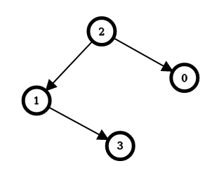
Input: n = 4, edges = [[2,0],[2,1],[1,3]]
Output: [1,1,0,2]
Explanation: The image above shows the graph formed by the edges.
For node 0: after reversing the edge [2,0], it is possible to reach any other node starting from node 0.
So, answer[0] = 1.
For node 1: after reversing the edge [2,1], it is possible to reach any other node starting from node 1.
So, answer[1] = 1.
For node 2: it is already possible to reach any other node starting from node 2.
So, answer[2] = 0.
For node 3: after reversing the edges [1,3] and [2,1], it is possible to reach any other node starting from node 3.
So, answer[3] = 2.
Example 2:
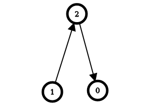
Input: n = 3, edges = [[1,2],[2,0]]
Output: [2,0,1]
Explanation: The image above shows the graph formed by the edges.
For node 0: after reversing the edges [2,0] and [1,2], it is possible to reach any other node starting from node 0.
So, answer[0] = 2.
For node 1: it is already possible to reach any other node starting from node 1.
So, answer[1] = 0.
For node 2: after reversing the edge [1, 2], it is possible to reach any other node starting from node 2.
So, answer[2] = 1.
Constraints:
2 <= n <= 105edges.length == n - 1edges[i].length == 20 <= ui == edges[i][0] < n0 <= vi == edges[i][1] < nui != vi- The input is generated such that if the edges were bi-directional, the graph would be a tree.
Approach Overview
Problem Overview: You are given a directed tree with n nodes. For each node, determine the minimum number of edge reversals required so every other node becomes reachable starting from that node. The output is an array where index i represents the minimum reversals needed if node i is treated as the root.
Approach 1: Reverse BFS Traversal (O(n) time, O(n) space)
Model each edge in both directions inside an adjacency list. The original direction has cost 0 and the reversed direction has cost 1. Run a Breadth-First Search from node 0 to count how many edges must be reversed so every node becomes reachable from this root. Each traversal accumulates the reversal cost based on edge direction. This produces the baseline number of reversals for node 0. The insight is that moving along an edge aligned with the direction requires no change, while going against it implies a reversal.
Approach 2: BFS Re-rooting Propagation (O(n) time, O(n) space)
After computing the reversal count for root 0, propagate results to all nodes using another BFS. When moving the root from node u to neighbor v, adjust the answer depending on edge orientation. If the original edge is u → v, re-rooting requires one extra reversal. If it is v → u, one reversal is saved. This local adjustment allows computing results for all nodes without recomputing the whole traversal. The graph is processed once, making it linear time.
Approach 3: Using BFS to Determine Minimum Edge Reversals from Root (O(n) time, O(n) space)
This variation focuses on computing the base cost from a single root using weighted traversal logic. Each edge contributes either 0 or 1 depending on whether it must be reversed relative to traversal direction. The algorithm iterates through neighbors and accumulates reversal costs while marking visited nodes. This approach isolates the core counting step and is useful before applying a re-rooting optimization.
Approach 4: Dynamic Programming with Tree Re-rooting (O(n) time, O(n) space)
Use Depth-First Search combined with a re-rooting technique often used in dynamic programming on trees. The first DFS calculates how many reversals are needed when node 0 is the root. A second DFS propagates results to children by adjusting counts depending on edge orientation. Re-rooting avoids recomputation by reusing parent results and modifying them with constant-time updates. This technique generalizes well to many tree DP problems where answers depend on the chosen root.
Recommended for interviews: The tree re-rooting dynamic programming approach is the expected optimal solution. It runs in linear time and demonstrates strong understanding of graph traversal and root transition logic. Starting with the BFS counting step helps clarify the problem, but implementing the re-rooting propagation shows deeper algorithmic skill.
Approach 1: Using BFS to Determine Minimum Edge Reversals from Root
This approach involves initially assuming node 0 as the starting root and calculating the minimum edge reversals needed to reach from node 0 to every other node. We first build an adjacency list, taking into account both forward and reverse edges, with a reverse edge counted as an additional cost of one for BFS traversal. Finally, we propagate the costs using BFS.
This Python solution uses a Breadth-First Search (BFS) to determine the minimum number of reversals needed to make all nodes reachable from the root (node 0). It builds an adjacency list representing the bidirectional edges, using a tuple to distinguish between forward and reverse edges by assigning a cost of 1 to reverse edges.
The BFS explores neighbors and adds them to the queue only if replacing the current path yields fewer reversals than previously recorded via a dynamic programming approach, ensuring all possibilities are explored while maintaining optimal substructure.
Functionally, it calculates and returns the result for each node as the minimum reversals needed for reachability from that node.
Code
Python
Complexity
Time Complexity: O(n), since each edge is processed only once in the BFS traversal.
Space Complexity: O(n), due to the storage requirement for the graph adjacency list and the min_reversals array.
Approach 2: Dynamic Programming with Tree Re-rooting
After calculating the minimum reversals needed from a fixed root (say node 0), we shift the root through each node. By analyzing the relationship between a node and its children, and leveraging already computed information from the original root, we can dynamically calculate the reversal cost for each node without recomputing from scratch.
In this Python implementation, we first assume node 0 as the root node and perform a DFS to visit each node from this root (node 0). During the DFS traversal, the minimum number of reversals from the root to each node is dynamically updated.
Through tree re-rooting, this implementation shifts the root node dynamically and recalculates the reversal counts. It leverages the costs already calculated on a parent node to efficiently compute the edge reversal cost for children nodes.
Code
Python
Complexity
Time Complexity: O(n), as DFS explores each node and edge once for all structural transformations.
Space Complexity: O(n), the space required mainly for the adjacency list and result storage.
Approach 3: Approach 1: Reverse BFS Traversal
The idea is to perform a reverse BFS traversal starting from each node, simulating the reversal of edges and calculating the required number of reversals.
Initially, consider reversing all the edges. Use Reverse BFS from each node to see how many reversals can be reverted back to the original direction and compute the minimal reversals needed.
We create an adjacency list where each edge appears as both directed and reversed. Using BFS, we traverse the graph starting from each node, updating the minimum reversal calculation based on edge directions. This provides the minimum number of reversals to reach all nodes from each starting node.
Complexity
Time Complexity: O(n), where n is the number of nodes, as each edge is visited a constant number of times.
Space Complexity: O(n), required for the adjacency list and BFS queue.
Approach 4: Approach 2: Dynamic Programming with DFS
Utilize a dynamic programming strategy with DFS to compute the answer by adopting a similar logic to the tree-diameter problem where we calculate the cost to traverse back to the starting node after visiting each other node.
This solution exploits the properties of DFS in a tree structure, calculating the minimum edge reversals by dynamically computing costs through recursive traversal. This approach is similar to tree-diameter problems.
Code
Java
JavaScript
Complexity
Time Complexity: O(n), as each node and edge is visited a constant number of times.
Space Complexity: O(n), used for the adjacency list and recursive call stack.
Approach 5: Default Approach
Code
Python
Java
C++
Go
TypeScript
Complexity Comparison
| Approach | Complexity |
|---|---|
| Using BFS to Determine Minimum Edge Reversals from Root | Time Complexity: O(n), since each edge is processed only once in the BFS traversal. Space Complexity: O(n), due to the storage requirement for the graph adjacency list and the min_reversals array. |
| Dynamic Programming with Tree Re-rooting | Time Complexity: O(n), as DFS explores each node and edge once for all structural transformations. Space Complexity: O(n), the space required mainly for the adjacency list and result storage. |
| Approach 1: Reverse BFS Traversal | Time Complexity: O(n), where n is the number of nodes, as each edge is visited a constant number of times. |
| Approach 2: Dynamic Programming with DFS | Time Complexity: O(n), as each node and edge is visited a constant number of times. |
| Default Approach | — |
Detailed Complexity Analysis
| Approach | Time | Space | When to Use |
|---|---|---|---|
| Reverse BFS Traversal | O(n) | O(n) | Compute base reversal count from a single root |
| BFS Re-rooting Propagation | O(n) | O(n) | Efficiently derive answers for all nodes after initial root computation |
| BFS Root Cost Calculation | O(n) | O(n) | Understanding the core reversal counting logic |
| Dynamic Programming with DFS (Tree Re-rooting) | O(n) | O(n) | Interview‑optimal solution for computing results for every node |
Video Solution
🔴 2858. Minimum Edge Reversals So Every Node Is Reachable II Graph II DP II Leetcode 2858 • Aryan Mittal • 7,346 views views
Watch 9 more video solutions →Frequently Asked Questions
Is Minimum Edge Reversals So Every Node Is Reachable easy or hard?
Minimum Edge Reversals So Every Node Is Reachable Python/Java solution
How to solve Minimum Edge Reversals So Every Node Is Reachable in O(n)?
What is the best approach for Minimum Edge Reversals So Every Node Is Reachable?
Is Minimum Edge Reversals So Every Node Is Reachable asked at Google/Amazon/Meta?
What data structure is used in Minimum Edge Reversals So Every Node Is Reachable?
What is the time complexity of Minimum Edge Reversals So Every Node Is Reachable?
Ready to solve this problem?
Practice Minimum Edge Reversals So Every Node Is Reachable with our built-in code editor and test cases.
Practice on FleetCodeProblem Info
Table of Contents
Practice this problem
Open in Editor