You are given an m x n integer matrix mat and an integer target.
Choose one integer from each row in the matrix such that the absolute difference between target and the sum of the chosen elements is minimized.
Return the minimum absolute difference.
The absolute difference between two numbers a and b is the absolute value of a - b.
Example 1:
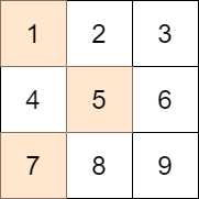
Input: mat = [[1,2,3],[4,5,6],[7,8,9]], target = 13
Output: 0
Explanation: One possible choice is to:
- Choose 1 from the first row.
- Choose 5 from the second row.
- Choose 7 from the third row.
The sum of the chosen elements is 13, which equals the target, so the absolute difference is 0.
Example 2:
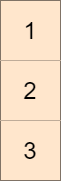
Input: mat = [[1],[2],[3]], target = 100
Output: 94
Explanation: The best possible choice is to:
- Choose 1 from the first row.
- Choose 2 from the second row.
- Choose 3 from the third row.
The sum of the chosen elements is 6, and the absolute difference is 94.
Example 3:
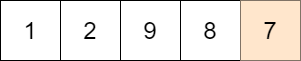
Input: mat = [[1,2,9,8,7]], target = 6
Output: 1
Explanation: The best choice is to choose 7 from the first row.
The absolute difference is 1.
Constraints:
m == mat.lengthn == mat[i].length1 <= m, n <= 701 <= mat[i][j] <= 701 <= target <= 800Problem Overview: You are given an m x n matrix and a target value. You must choose exactly one element from each row. The goal is to minimize |sum - target|, where sum is the total of the chosen elements.
Approach 1: Backtracking with Pruning (Exponential, worst-case O(n^m) time, O(m) space)
This approach tries every possible combination by selecting one element from each row using recursion. At each step, you add the chosen value to the current sum and move to the next row. A pruning rule cuts off branches when the current sum already exceeds a threshold where improvement is impossible. Sorting row values and stopping early once sums grow too large significantly reduces the search space in practice. The method is straightforward and works well for smaller matrices but can still degrade toward exponential complexity in the worst case.
Approach 2: Dynamic Programming with Closure Check (O(m * n * S) time, O(S) space)
The optimal solution uses dynamic programming to track reachable sums after processing each row. Start with a set containing 0. For every row, iterate through the current sums and add each element in that row, generating the next set of possible sums. To prevent the state space from exploding, apply a closure check: cap the sums at a reasonable bound around the target (for example target + 70, since matrix values are small). This pruning keeps the DP state compact while still preserving all sums that could produce the optimal difference.
The key insight: the exact sum doesn't matter once it grows far beyond the target. Only sums within a limited range can produce the minimum absolute difference. Using a boolean array or hash set to represent reachable sums keeps transitions fast. Each row performs a simple nested iteration over current sums and row elements, making the implementation clean and predictable.
This technique is a classic pattern for subset-style problems where the number of combinations is large but the sum range is bounded. It appears frequently in array and matrix problems that involve selecting elements under constraints.
Recommended for interviews: Dynamic programming with closure checking. Interviewers expect you to recognize that brute-force combinations are too large and convert the problem into a bounded sum DP. Showing the backtracking approach first demonstrates problem understanding, but the DP optimization shows stronger algorithmic thinking.
This approach uses a dynamic programming table to keep track of all possible sums we can achieve with the elements from the first i rows up to a certain maximum value. At each row, we add each number in that row to all possible sums from the previous row, ensuring to keep the solutions optimized by only storing possible sums that bring us closer to the target.
This Python function iterates through each row of the matrix, calculating all the possible sums one can generate using numbers up to the current row. The goal is to find the sum that leads to the smallest absolute difference from the target. By working through each row, we use a set to ensure unique and possible sums, thereby optimizing our calculations.
Time Complexity: O(m * n * n) because for each of the m rows, we're recalculating across n elements with the running sum set of at most n growth in complexity terms. Space Complexity: O(kn) where k is the maximum possible sum trackable at each step, kept within practical limits by problem constraints.
This approach utilizes backtracking to explore each possible selection choice exhaustively and prune unneeded branches. It builds sums row by row and branches only when potential can minimize the absolute target difference calculated dynamically.
This Java solution implements backtracking by recursively choosing each row's elements to form a sum. It uses memoization to avoid recalculating previously explored states, thus pruning unnecessary calculations and enhancing efficiency.
Java
JavaScript
Time Complexity: O(n^m), because each choice might lead to all subsequent options. Space Complexity: O(m * t), employing a basic memoization table dependent on target constraint values for optimization.
Let f[i][j] represent whether it is possible to select elements from the first i rows with a sum of j. Then we have the state transition equation:
$
f[i][j] = \begin{cases} 1 & if there exists x \in row[i] such that f[i - 1][j - x] = 1 \ 0 & otherwise \end{cases}
where row[i] represents the set of elements in the i-th row.
Since f[i][j] is only related to f[i - 1][j], we can use a rolling array to optimize the space complexity.
Finally, we traverse the f array to find the smallest absolute difference.
The time complexity is O(m^2 times n times C) and the space complexity is O(m times C). Here, m and n are the number of rows and columns of the matrix, respectively, and C$ is the maximum value of the matrix elements.
| Approach | Complexity |
|---|---|
| Dynamic Programming with Closure Check | Time Complexity: O(m * n * n) because for each of the m rows, we're recalculating across n elements with the running sum set of at most n growth in complexity terms. Space Complexity: O(kn) where k is the maximum possible sum trackable at each step, kept within practical limits by problem constraints. |
| Backtracking with Pruning | Time Complexity: O(n^m), because each choice might lead to all subsequent options. Space Complexity: O(m * t), employing a basic memoization table dependent on target constraint values for optimization. |
| Dynamic Programming (Grouped Knapsack) | — |
| Approach | Time | Space | When to Use |
|---|---|---|---|
| Backtracking with Pruning | O(n^m) worst case | O(m) | Useful for understanding the brute-force search and when matrix size is small |
| Dynamic Programming with Closure Check | O(m * n * S) | O(S) | Best general solution when sum range is bounded around the target |
LeetCode 1981. Minimize the Difference Between Target and Chosen Elements • Happy Coding • 2,560 views views
Watch 6 more video solutions →Practice Minimize the Difference Between Target and Chosen Elements with our built-in code editor and test cases.
Practice on FleetCode