You are given an m x n integer matrix points (0-indexed). Starting with 0 points, you want to maximize the number of points you can get from the matrix.
To gain points, you must pick one cell in each row. Picking the cell at coordinates (r, c) will add points[r][c] to your score.
However, you will lose points if you pick a cell too far from the cell that you picked in the previous row. For every two adjacent rows r and r + 1 (where 0 <= r < m - 1), picking cells at coordinates (r, c1) and (r + 1, c2) will subtract abs(c1 - c2) from your score.
Return the maximum number of points you can achieve.
abs(x) is defined as:
x for x >= 0.-x for x < 0.
Example 1:

Input: points = [[1,2,3],[1,5,1],[3,1,1]]
Output: 9
Explanation:
The blue cells denote the optimal cells to pick, which have coordinates (0, 2), (1, 1), and (2, 0).
You add 3 + 5 + 3 = 11 to your score.
However, you must subtract abs(2 - 1) + abs(1 - 0) = 2 from your score.
Your final score is 11 - 2 = 9.
Example 2:
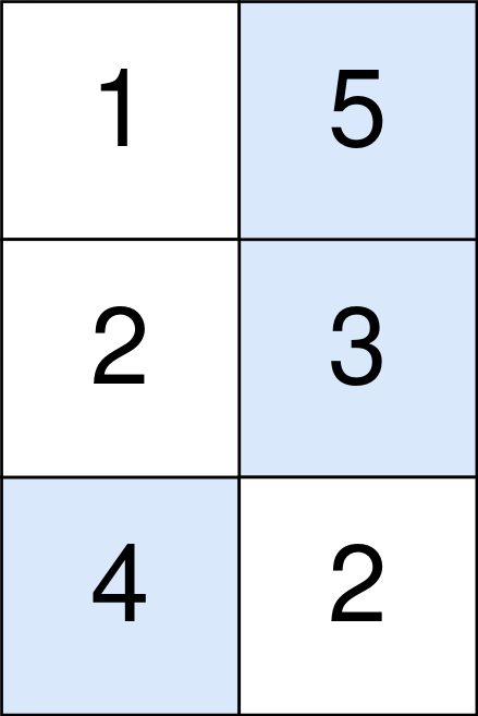
Input: points = [[1,5],[2,3],[4,2]]
Output: 11
Explanation:
The blue cells denote the optimal cells to pick, which have coordinates (0, 1), (1, 1), and (2, 0).
You add 5 + 3 + 4 = 12 to your score.
However, you must subtract abs(1 - 1) + abs(1 - 0) = 1 from your score.
Your final score is 12 - 1 = 11.
Constraints:
m == points.lengthn == points[r].length1 <= m, n <= 1051 <= m * n <= 1050 <= points[r][c] <= 105Problem Overview: You get an m x n matrix where selecting a cell in each row earns its value, but moving between columns costs |c1 - c2|. The goal is to maximize the total score while picking exactly one column per row.
Approach 1: Dynamic Programming with Direct Transition (O(m * n^2) time, O(n) space)
Define dp[j] as the maximum points achievable when selecting column j in the current row. For every row, compute the new value for each column by checking every column from the previous row: dp_new[j] = points[i][j] + max(dp[k] - |j - k|) for all k. This brute-force transition explicitly evaluates the movement penalty between columns. It is straightforward and clearly expresses the state transition, but the nested loop over columns makes it O(n^2) per row. This approach works for smaller matrices but becomes slow when n grows large.
Approach 2: Dynamic Programming with Two Pass Strategy (O(m * n) time, O(n) space)
The key observation: the transition dp[k] - |j - k| can be split into two directional cases. When k ≤ j, the cost becomes dp[k] + k - j. When k ≥ j, it becomes dp[k] - k + j. This allows you to precompute running maximum values while scanning the row from left-to-right and right-to-left. During the left pass, maintain best = max(best, dp[j] + j) and compute candidate scores. During the right pass, maintain best = max(best, dp[j] - j). Combining these passes gives the optimal transition for every column in linear time. This reduces each row update from quadratic to linear complexity.
Approach 3: Dynamic Programming with Optimized Transition State (O(m * n) time, O(n) space)
This implementation expresses the same optimization more compactly by propagating the best reachable values while iterating across the row. Instead of recomputing |j - k|, you carry forward the best previous score adjusted by movement cost. The technique relies on maintaining rolling maximums and updating them as the column index changes. It produces the same optimal DP state but with fewer temporary structures and cleaner transitions. Many competitive programmers prefer this formulation because the code is shorter while preserving the O(mn) runtime.
Recommended for interviews: Start by describing the direct dynamic programming transition to demonstrate you understand the state definition and movement penalty. Then optimize it using the two-pass trick. Interviewers expect the O(mn) DP solution because it shows you can transform a quadratic transition into a linear scan using prefix maximums. This pattern appears frequently in dynamic programming problems on grids and matrix traversal, especially when working with column-distance penalties inside array-based states.
This approach uses dynamic programming where we keep track of the maximum points obtainable for each cell using two linear passes per row: one from left to right and the other from right to left. This ensures that we account for the cost of moving between rows efficiently.
The solution uses two arrays, leftToRight and rightToLeft, to keep track of the running maximum of points at each cell considering the point loss moving horizontally. The maximum value for each cell in the current row is calculated by combining the respective running maximum from leftToRight and rightToLeft plus the points from the current cell.
Time Complexity: O(m * n) as we iterate through the cells twice per row. Space Complexity: O(n) due to the auxiliary arrays used.
This approach uses a dynamic array to store optimal points value and computes it via a prefix and suffix maximum accumulations, thereby reducing the transition complexity while still making sure every cell's deduction is feasible within two linear passes.
This variation keeps the dynamic arrays leftMax and rightMax for efficient transitions between rows to directly adjust the prefix-suffix maximum pairs.
Time Complexity: O(m * n). Space Complexity: O(n), reducing allocation per row iteration.
Python
Java
C++
Go
TypeScript
| Approach | Complexity |
|---|---|
| Dynamic Programming with Two Pass Strategy | Time Complexity: O(m * n) as we iterate through the cells twice per row. Space Complexity: O(n) due to the auxiliary arrays used. |
| Dynamic Programming with Optimized Transition State | Time Complexity: O(m * n). Space Complexity: O(n), reducing allocation per row iteration. |
| Default Approach | — |
| Approach | Time | Space | When to Use |
|---|---|---|---|
| Dynamic Programming with Direct Transition | O(m * n^2) | O(n) | Useful for understanding the DP state and transition before optimizing |
| Dynamic Programming with Two Pass Strategy | O(m * n) | O(n) | Optimal solution for large matrices and typical interview expectations |
| DP with Optimized Transition State | O(m * n) | O(n) | Cleaner implementation of the optimized DP using rolling maximums |
Maximum Number of Points with Cost - Leetcode 1937 - Python • NeetCodeIO • 21,874 views views
Watch 9 more video solutions →Practice Maximum Number of Points with Cost with our built-in code editor and test cases.
Practice on FleetCode