You are given an image represented by an m x n grid of integers image, where image[i][j] represents the pixel value of the image. You are also given three integers sr, sc, and color. Your task is to perform a flood fill on the image starting from the pixel image[sr][sc].
To perform a flood fill:
color.Return the modified image after performing the flood fill.
Example 1:
Input: image = [[1,1,1],[1,1,0],[1,0,1]], sr = 1, sc = 1, color = 2
Output: [[2,2,2],[2,2,0],[2,0,1]]
Explanation:
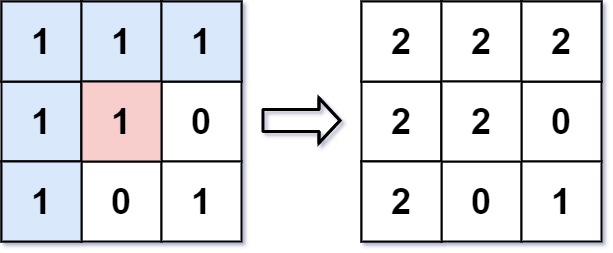
From the center of the image with position (sr, sc) = (1, 1) (i.e., the red pixel), all pixels connected by a path of the same color as the starting pixel (i.e., the blue pixels) are colored with the new color.
Note the bottom corner is not colored 2, because it is not horizontally or vertically connected to the starting pixel.
Example 2:
Input: image = [[0,0,0],[0,0,0]], sr = 0, sc = 0, color = 0
Output: [[0,0,0],[0,0,0]]
Explanation:
The starting pixel is already colored with 0, which is the same as the target color. Therefore, no changes are made to the image.
Constraints:
m == image.lengthn == image[i].length1 <= m, n <= 500 <= image[i][j], color < 2160 <= sr < m0 <= sc < nProblem Overview: You are given a 2D image where each cell represents a pixel color. Starting from a specific pixel (sr, sc), change its color and all 4-directionally connected pixels with the same original color to a new color. The task is essentially traversing a connected component in a grid.
Approach 1: Recursive Depth-First Search (DFS) (Time: O(m*n), Space: O(m*n))
This approach treats the grid as a graph and performs a recursive DFS from the starting cell. First store the original color at (sr, sc). If the new color is the same as the original, return immediately to avoid infinite recursion. Otherwise, recursively explore the four directions (up, down, left, right). Whenever a neighboring cell has the same original color, update it and continue the DFS. Each cell is visited at most once, giving O(m*n) time for an image of size m x n. The recursion stack can grow up to the size of the connected region, resulting in O(m*n) space in the worst case. This method is simple and maps naturally to problems involving Depth-First Search on a matrix.
Approach 2: Iterative Breadth-First Search (BFS) (Time: O(m*n), Space: O(m*n))
The BFS approach performs the same region traversal but uses a queue instead of recursion. Start by pushing the initial pixel into a queue and recolor it. While the queue is not empty, pop a cell and examine its four neighbors. If a neighbor lies within bounds and has the original color, recolor it and push it into the queue. BFS expands level by level across the connected component, ensuring every valid pixel is processed exactly once. Time complexity remains O(m*n) because each pixel is enqueued and processed at most once. Space complexity is also O(m*n) due to the queue in the worst case when the entire grid belongs to the same region. This approach is useful when recursion depth might be large and iterative control is preferred, especially in problems involving Breadth-First Search over an array-backed grid.
Recommended for interviews: The recursive DFS solution is the most common answer because it is concise and clearly demonstrates understanding of grid traversal. Interviewers typically expect you to recognize the problem as a connected component search. Mentioning both DFS and BFS shows strong fundamentals: DFS demonstrates recursion and graph traversal intuition, while BFS shows awareness of iterative alternatives and stack depth limitations.
This approach uses recursion to explore all connected pixels that need to be updated. Starting from the initial pixel, you recursively attempt to update all four possible directions (up, down, left, right) whenever the neighboring pixel has the same original color.
The recursion ensures that all connected and valid pixels are eventually updated. Make sure to handle the base case where the function stops if the pixel is out of bounds or if it doesn't need updating (either because it's already updated or has a different color).
In this Python solution, we define a recursive function dfs which updates the color of a pixel and then recursively calls itself for each adjacent pixel. The function checks boundary conditions and whether the pixel is of the original color before updating it.
Time Complexity: O(m * n) because in the worst case, all of the pixels will be connected and thus changed.
Space Complexity: O(m * n) due to the recursion call stack.
This approach employs an iterative breadth-first search (BFS) using a queue. Starting from the initial pixel, we enqueue it and begin the BFS process, updating connected pixels of the same original color to the new color.
For each pixel, check its adjacent pixels and enqueue them if they are valid and of the original color. This continues until the queue is empty, ensuring all pixels are updated appropriately.
This Python solution uses a queue to implement the BFS process, iterating over each pixel and its adjacent pixels. The queue ensures all connected pixels are enqueued and processed correctly.
Time Complexity: O(m * n), where m and n are the dimensions of the image (same as DFS).
Space Complexity: O(m * n), as we may store all pixels in the queue in the worst-case scenario.
We denote the initial pixel's color as oc. If oc is not equal to the target color color, we start a depth-first search from (sr, sc) to change the color of all eligible pixels to the target color.
The time complexity is O(m times n), and the space complexity is O(m times n). Here, m and n are the number of rows and columns of the 2D array image, respectively.
We first check if the initial pixel's color is equal to the target color. If it is, we return the original image directly. Otherwise, we can use the breadth-first search method, starting from (sr, sc), to change the color of all eligible pixels to the target color.
Specifically, we define a queue q and add the initial pixel (sr, sc) to the queue. Then, we continuously take pixels (i, j) from the queue, change their color to the target color, and add the pixels in the four directions (up, down, left, right) that have the same original color as the initial pixel to the queue. When the queue is empty, we have completed the flood fill.
The time complexity is O(m times n), and the space complexity is O(m times n). Here, m and n are the number of rows and columns of the 2D array image, respectively.
| Approach | Complexity |
|---|---|
| Recursive Depth-First Search (DFS) Approach | Time Complexity: O(m * n) because in the worst case, all of the pixels will be connected and thus changed. |
| Iterative Breadth-First Search (BFS) Approach | Time Complexity: O(m * n), where m and n are the dimensions of the image (same as DFS). |
| DFS | — |
| BFS | — |
| Approach | Time | Space | When to Use |
|---|---|---|---|
| Recursive DFS | O(m*n) | O(m*n) | Best for concise implementation and typical interview solutions involving recursive grid traversal |
| Iterative BFS | O(m*n) | O(m*n) | Useful when avoiding recursion depth limits or when iterative queue-based traversal is preferred |
LeetCode 733. Flood Fill (Algorithm Explained) • Nick White • 66,336 views views
Watch 9 more video solutions →Practice Flood Fill with our built-in code editor and test cases.
Practice on FleetCodePractice this problem
Open in Editor