
Count the Number of Complete Components - Solution & Explanation
Problem Statement
You are given an integer n. There is an undirected graph with n vertices, numbered from 0 to n - 1. You are given a 2D integer array edges where edges[i] = [ai, bi] denotes that there exists an undirected edge connecting vertices ai and bi.
Return the number of complete connected components of the graph.
A connected component is a subgraph of a graph in which there exists a path between any two vertices, and no vertex of the subgraph shares an edge with a vertex outside of the subgraph.
A connected component is said to be complete if there exists an edge between every pair of its vertices.
Example 1:
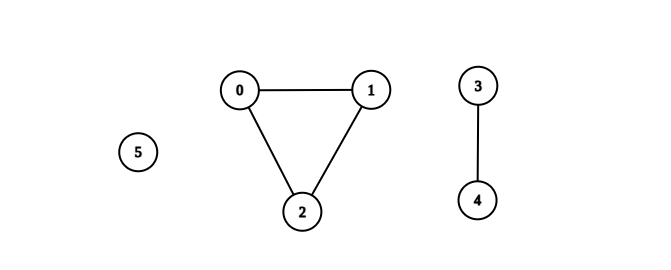
Input: n = 6, edges = [[0,1],[0,2],[1,2],[3,4]]
Output: 3
Explanation: From the picture above, one can see that all of the components of this graph are complete.
Example 2:
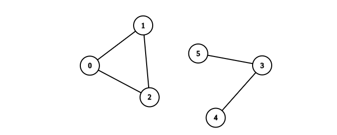
Input: n = 6, edges = [[0,1],[0,2],[1,2],[3,4],[3,5]]
Output: 1
Explanation: The component containing vertices 0, 1, and 2 is complete since there is an edge between every pair of two vertices. On the other hand, the component containing vertices 3, 4, and 5 is not complete since there is no edge between vertices 4 and 5. Thus, the number of complete components in this graph is 1.
Constraints:
1 <= n <= 500 <= edges.length <= n * (n - 1) / 2edges[i].length == 20 <= ai, bi <= n - 1ai != bi- There are no repeated edges.
Approach Overview
Problem Overview: You are given an undirected graph with n nodes and a list of edges. The task is to count how many connected components are complete graphs. A component is complete when every pair of distinct nodes inside it has an edge between them. For a component with k nodes, the total number of edges must be k * (k - 1) / 2.
Approach 1: Using Sorting (O(E log E) time, O(E) space)
This method starts by sorting the edge list so that edges belonging to the same node range appear together. After sorting, you iterate through the edges and group nodes into components while counting how many edges belong to each group. For every component discovered, track two values: the number of nodes and the number of edges encountered. Once traversal for a component finishes, compute the expected edge count using k * (k - 1) / 2. If the actual edge count matches this value, the component is complete. Sorting makes it easier to process related edges sequentially and simplifies component grouping when the edge list is large or initially unordered.
Approach 2: Using a Hash Map (O(V + E) time, O(V + E) space)
This approach builds an adjacency list using a hash map where each node maps to its neighbors. Then traverse the graph using Depth-First Search or Breadth-First Search to explore one connected component at a time. During traversal, count how many nodes belong to the component and sum the degrees of those nodes. Since each undirected edge contributes twice to the degree count, divide the total degree by two to get the actual edge count. After finishing the traversal, verify whether the component satisfies the complete graph condition edges == k * (k - 1) / 2. Hash map adjacency lists provide constant-time neighbor lookups and make this method scale well for sparse graphs.
This problem is fundamentally a connected component analysis task combined with a mathematical property of complete graphs. Graph traversal guarantees that every node in a component is visited exactly once. The edge-count validation step ensures that the component is fully connected internally. Similar ideas appear in problems involving graph validation and connectivity checks, often implemented with Union Find or DFS.
Recommended for interviews: The hash map + DFS/BFS approach is the expected solution. It runs in linear time O(V + E) and demonstrates clear understanding of graph traversal and component analysis. The sorting-based approach works but adds unnecessary overhead due to O(E log E) sorting. Showing the traversal solution signals stronger graph fundamentals.
Approach 1: Approach 1: Using Sorting
This approach involves sorting the array and then finding the target element based on the problem's requirement. Sorting simplifies many search operations by arranging the elements in a predetermined order.
This C program sorts an array and then searches for a target element. The qsort function is used for sorting, providing a fast O(n log n) solution. After sorting, a linear search is performed to find the target element, which can be optimized further.
Complexity
Time Complexity: O(n log n) due to sorting
Space Complexity: O(1) as it sorts in place
Approach 2: Approach 2: Using a Hash Map
This approach leverages a hash map for quick look-up times. By storing elements in a hash map with their indices, we can reduce the time complexity for look-up operations significantly.
This C implementation uses a simple hash map to find elements quickly. The hash map provides an average time complexity of O(1) for both insertion and lookup, making this approach efficient for large inputs.
Complexity
Time Complexity: O(n) for building the map
Space Complexity: O(n) for map storage
Approach 3: Default Approach
Try this approach in the editor →Approach 4: Simple Method
Problems needed to solve:
- How do we maintain the link state between each node and the others? 如
- How can one determine whether multiple points form a connected graph?
For the first one: we can maintain each node's connection set(including itself).
For the second one: After solving the first one, we can see:
- the node itself includes every node in the connected graph(including itself).
- and only connected to the nodes in the connected graph.
Take example 1 to explain:
- Node 5's connected node is itself, so it is a connected graph.
- Node 0's connected 0, 1, 2. Same as nodes 1, 2.
- Nodes 3 and 4 also include themselves and each other.
Code
C++
Complexity Comparison
| Approach | Complexity |
|---|---|
| Approach 1: Using Sorting | Time Complexity: O(n log n) due to sorting |
| Approach 2: Using a Hash Map | Time Complexity: O(n) for building the map |
| Default Approach | — |
| Simple Method | — |
Detailed Complexity Analysis
| Approach | Time | Space | When to Use |
|---|---|---|---|
| Using Sorting | O(E log E) | O(E) | When edges must be processed in ordered groups or the input edge list is highly unordered |
| Using Hash Map + DFS/BFS | O(V + E) | O(V + E) | Best general solution for graph traversal and connected component detection |
Video Solution
Count the Number of Complete Components | Multiple Approaches | Leetcode 2685 | codestorywithMIK • codestorywithMIK • 12,315 views views
Watch 9 more video solutions →Frequently Asked Questions
Is Count the Number of Complete Components easy or hard?
Count the Number of Complete Components Python/Java solution
How to solve Count the Number of Complete Components in O(n)?
What is the best approach for Count the Number of Complete Components?
Is Count the Number of Complete Components asked at Google/Amazon/Meta?
What data structure is used in Count the Number of Complete Components?
What is the time complexity of Count the Number of Complete Components?
Ready to solve this problem?
Practice Count the Number of Complete Components with our built-in code editor and test cases.
Practice on FleetCode