Cat and Mouse II - Solution & Explanation

Q: Is Cat and Mouse II easy or hard?

Cat and Mouse II is classified as a Hard problem on LeetCode. It requires combining grid traversal, game theory reasoning, dynamic programming over states, and careful handling of cycles or repeated positions.

Q: Cat and Mouse II Python/Java solution

Python implementations usually use DFS with memoization and a state cache keyed by mouse position, cat position, and turn. Java and C++ solutions often implement BFS with state tracking and degree counting to perform retrograde analysis over the game graph.

Q: How to solve Cat and Mouse II in O(n)?

An O(n) solution is not feasible because the game state depends on both mouse and cat positions. The minimum state space is roughly (m*n)^2 with an additional turn dimension. Efficient solutions reduce the search using memoization or BFS-based retrograde analysis over the state graph.

Q: What is the best approach for Cat and Mouse II?

The most common approach is minimax with memoization. Each game state is defined by the mouse position, cat position, and whose turn it is. DFS explores all possible moves while caching results to avoid recomputation. This converts the adversarial game into a dynamic programming problem over states.

Q: Is Cat and Mouse II asked at Google/Amazon/Meta?

Game theory and adversarial search problems like Cat and Mouse II appear in interviews at companies such as Google, Meta, and Amazon. While the exact problem may not appear frequently, the techniques—minimax search, memoization, and graph state modeling—are common interview topics.

Q: What data structure is used in Cat and Mouse II?

The solution relies on grids, graph-style state representations, and memoization tables or DP arrays. DFS recursion with caching or BFS queues are typically used to evaluate game states and propagate winning or losing outcomes.

Q: What is the time complexity of Cat and Mouse II?

The typical solution runs in about O((m*n)^2 * K), where m*n represents grid cells and K is the maximum number of turns considered (often capped near 1000). The state space includes mouse position, cat position, and turn. Memoization or BFS state pruning prevents exponential exploration.

HardArray Math Dynamic Programming Graph34 min readAsked at: Google

Practice this problem

Problem Statement

A game is played by a cat and a mouse named Cat and Mouse.

The environment is represented by a grid of size rows x cols, where each element is a wall, floor, player (Cat, Mouse), or food.

Players are represented by the characters 'C'(Cat),'M'(Mouse).
Floors are represented by the character '.' and can be walked on.
Walls are represented by the character '#' and cannot be walked on.
Food is represented by the character 'F' and can be walked on.
There is only one of each character 'C', 'M', and 'F' in grid.

Mouse and Cat play according to the following rules:

Mouse moves first, then they take turns to move.
During each turn, Cat and Mouse can jump in one of the four directions (left, right, up, down). They cannot jump over the wall nor outside of the grid.
catJump, mouseJump are the maximum lengths Cat and Mouse can jump at a time, respectively. Cat and Mouse can jump less than the maximum length.
Staying in the same position is allowed.
Mouse can jump over Cat.

The game can end in 4 ways:

If Cat occupies the same position as Mouse, Cat wins.
If Cat reaches the food first, Cat wins.
If Mouse reaches the food first, Mouse wins.
If Mouse cannot get to the food within 1000 turns, Cat wins.

Given a rows x cols matrix grid and two integers catJump and mouseJump, return true if Mouse can win the game if both Cat and Mouse play optimally, otherwise return false.

Example 1:

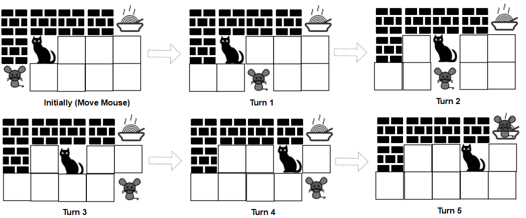
Input: grid = ["####F","#C...","M...."], catJump = 1, mouseJump = 2
Output: true
Explanation: Cat cannot catch Mouse on its turn nor can it get the food before Mouse.

Example 2:

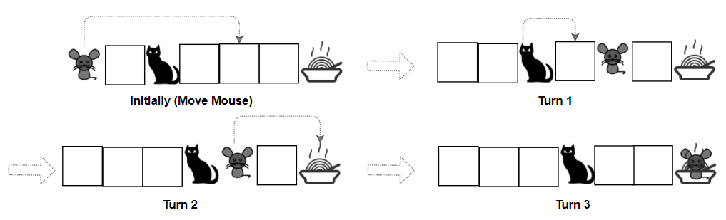
Input: grid = ["M.C...F"], catJump = 1, mouseJump = 4
Output: true

Example 3:

Input: grid = ["M.C...F"], catJump = 1, mouseJump = 3
Output: false

Constraints:

rows == grid.length
cols = grid[i].length
1 <= rows, cols <= 8
grid[i][j] consist only of characters 'C', 'M', 'F', '.', and '#'.
There is only one of each character 'C', 'M', and 'F' in grid.
1 <= catJump, mouseJump <= 8

Approach Overview

Problem Overview: A mouse and a cat move on a grid containing walls, food, and empty cells. The mouse moves first and both players can jump several cells in one direction. The mouse wins if it reaches the food, the cat wins if it catches the mouse or reaches the food first. The challenge is determining whether the mouse can force a win assuming both players play optimally.

Approach 1: Minimax with Memoization (Game DFS) (Time: O((mn)^2 * K), Space: O((mn)^2 * K))

This approach models the game as a recursive minimax search. Each state is defined by the mouse position, cat position, and whose turn it is. From a state, generate all valid moves by iterating up to the maximum jump distance in the four directions until hitting a wall. The mouse tries to reach the food or move into a state where the cat eventually loses, while the cat tries to capture the mouse or force a losing state for the mouse. Use memoization to cache results for previously evaluated states to avoid exponential recomputation. A move counter (usually capped around 1000 turns) prevents infinite loops. This turns a huge game tree into a manageable dynamic programming problem over states. The technique combines ideas from game theory and dynamic programming.

Approach 2: Breadth-First Search with State Tracking (Retrograde Analysis) (Time: O((mn)^2 * K), Space: O((mn)^2 * K))

This solution treats the game as a directed graph where each node represents a full state: (mousePosition, catPosition, turn). Instead of exploring forward, it performs retrograde analysis using BFS from known terminal states. Terminal states include the mouse reaching food (mouse win) or the cat catching the mouse (cat win). Maintain degree counts for each state representing how many moves are still unresolved. When a state is determined to be winning for one player, propagate that result backward to predecessor states. If all moves from a predecessor lead to opponent wins, that state becomes a loss. This technique resembles topological sorting on the state graph and avoids deep recursion. It works well for large state spaces typical in graph game problems.

Recommended for interviews: Minimax with memoization is the most intuitive approach and clearly demonstrates understanding of game states and optimal play. Interviewers often expect you to identify the state definition and apply DFS with caching. The BFS retrograde method is more advanced and efficient for reasoning about large game graphs, showing deeper understanding of graph processing and competitive game analysis.

Approach 1: Minimax with Memoization

In this approach, we use a recursive minimax strategy with memoization to simulate the game turns. The strategy checks all possible moves for both players and assumes that they play optimally. The goal is to determine if there is a path that allows the Mouse to win before the Cat can win.

We recursively compute the result for each state — characterized by the positions of Cat, Mouse, and the turn number — and store the results to avoid redundant computations.

This solution uses a DFS-like approach with memoization to minimize repeated calculations. We first parse the grid to find the initial positions of the cat, mouse, and food. The recursive function dp simulates the game, considering moves for both players and deciding the result of the game with optimal play from both sides. The memoization is achieved using the lru_cache decorator, which stores the result of each state configuration.

Code

Python JavaScript

Python

JavaScript

Complexity

Time Complexity: O(n^4) due to recursive state space exploration up to a depth of 1000 moves potential.

Space Complexity: O(n^4) because of memoization of the states, where n is the number of grid cells.

Try this approach in the editor →

Approach 2: Breadth-First Search with State Tracking

In this approach, we use a Breadth-First Search (BFS) strategy to systematically explore the game states. By using a queue to store each game state, we can track the minimum number of moves needed for the Mouse to reach the food while avoiding the Cat.

Each state is represented by the positions of the Cat, Mouse, and the number of turns, ensuring that we explore all possible moves within 1000 turns. We keep track of visited states to reduce redundant processing.

This Java code implements a BFS strategy using a queue to explore each possible state. We parse the grid to identify initial positions, enqueuing the initial state. By exploring each direction for both cat and mouse moves, while considering optimal moves, we determine the earliest possible win condition for the Mouse.

Code

Java C++

Java

C++

Complexity

Time Complexity: O(n^4) as we explore potential grid configurations extensively within the move constraint.

Space Complexity: O(n^4) because of the queue storage for state exploration.

Try this approach in the editor →

Approach 3: Topological Sorting

According to the problem description, the state of the game is determined by the mouse's position, the cat's position, and whose turn it is. The following states can be determined directly:

When the cat and the mouse are at the same position, the cat wins — this is a winning state for the cat and a losing state for the mouse.
When the cat reaches the food first, the cat wins — this is a winning state for the cat and a losing state for the mouse.
When the mouse reaches the food first, the mouse wins — this is a winning state for the mouse and a losing state for the cat.

To determine the result of the initial state, we need to traverse all states starting from the boundary states. Each state contains the mouse's position, the cat's position, and whose turn it is. From the current state, we can derive all possible previous states: the mover in the previous state is the opposite of the current mover, and the mover's position in the previous state differs from that in the current state.

We use the tuple (m, c, t) to represent the current state, and (pm, pc, pt) to represent a possible previous state. All possible previous states are:

If the current mover is the mouse, then the previous mover was the cat, the mouse's position in the previous state equals the current mouse position, and the cat's position in the previous state is any neighbor of the current cat position.
If the current mover is the cat, then the previous mover was the mouse, the cat's position in the previous state equals the current cat position, and the mouse's position in the previous state is any neighbor of the current mouse position.

Initially, except for the boundary states, the results of all other states are unknown. Starting from the boundary states, for each state we derive all possible previous states and update their results according to the following logic:

If the previous mover is the same as the current winner, then the previous mover can reach the current state and win — directly update the previous state to the current winner.
If the previous mover is different from the current winner, and all states reachable by the previous mover are losing states for the previous mover, then we update the previous state to the current winner.

For the second update rule, we need to record the degree of each state. Initially, the degree of a state represents the number of nodes the mover of that state can move to, i.e., the number of neighbors of the node where the mover is located. If the mover is the cat and the cat's node is adjacent to the hole, the degree of that state should be decremented by 1.

When all states have been updated, the result of the initial state is the final answer.

The time complexity is O(m^2 times n^2 times (m + n)) and the space complexity is O(m^2 times n^2), where m and n are the number of rows and columns of the grid, respectively.

Code

Python Java C++Go TypeScript Rust

Python

Java

C++

TypeScript

Rust

Try this approach in the editor →

Complexity Comparison

Approach	Complexity
Minimax with Memoization	Time Complexity: O(n^4) due to recursive state space exploration up to a depth of 1000 moves potential. Space Complexity: O(n^4) because of memoization of the states, where n is the number of grid cells.
Breadth-First Search with State Tracking	Time Complexity: O(n^4) as we explore potential grid configurations extensively within the move constraint. Space Complexity: O(n^4) because of the queue storage for state exploration.
Topological Sorting	—

Detailed Complexity Analysis

Approach	Time	Space	When to Use
Minimax with Memoization	O((mn)^2 * K)	O((mn)^2 * K)	Best conceptual approach for interviews when modeling adversarial games
BFS with State Tracking (Retrograde Analysis)	O((mn)^2 * K)	O((mn)^2 * K)	Useful for large game graphs where backward propagation avoids deep recursion

Video Solution

LeetCode 1728. Cat and Mouse II • Happy Coding • 1,541 views views

Watch 7 more video solutions →

Frequently Asked Questions

Is Cat and Mouse II easy or hard?

Cat and Mouse II is classified as a Hard problem on LeetCode. It requires combining grid traversal, game theory reasoning, dynamic programming over states, and careful handling of cycles or repeated positions.

Cat and Mouse II Python/Java solution

Python implementations usually use DFS with memoization and a state cache keyed by mouse position, cat position, and turn. Java and C++ solutions often implement BFS with state tracking and degree counting to perform retrograde analysis over the game graph.

How to solve Cat and Mouse II in O(n)?

An O(n) solution is not feasible because the game state depends on both mouse and cat positions. The minimum state space is roughly (m*n)^2 with an additional turn dimension. Efficient solutions reduce the search using memoization or BFS-based retrograde analysis over the state graph.

What is the best approach for Cat and Mouse II?

The most common approach is minimax with memoization. Each game state is defined by the mouse position, cat position, and whose turn it is. DFS explores all possible moves while caching results to avoid recomputation. This converts the adversarial game into a dynamic programming problem over states.

Is Cat and Mouse II asked at Google/Amazon/Meta?

Game theory and adversarial search problems like Cat and Mouse II appear in interviews at companies such as Google, Meta, and Amazon. While the exact problem may not appear frequently, the techniques—minimax search, memoization, and graph state modeling—are common interview topics.

What data structure is used in Cat and Mouse II?

The solution relies on grids, graph-style state representations, and memoization tables or DP arrays. DFS recursion with caching or BFS queues are typically used to evaluate game states and propagate winning or losing outcomes.

What is the time complexity of Cat and Mouse II?

The typical solution runs in about O((m*n)^2 * K), where m*n represents grid cells and K is the maximum number of turns considered (often capped near 1000). The state space includes mouse position, cat position, and turn. Memoization or BFS state pruning prevents exponential exploration.

Ready to solve this problem?

Practice Cat and Mouse II with our built-in code editor and test cases.

Practice on FleetCode

Cat and Mouse

Escape The Ghosts

Problem Info

DifficultyHard

Acceptance40.4%

Approaches3

Reading time34 min

Asked at

Google

Practice this problem

Open in Editor

Cat and Mouse II - Solution & Explanation

Problem Statement

Approach Overview

Approach 1: Minimax with Memoization

Code

Complexity

Approach 2: Breadth-First Search with State Tracking

Code

Complexity

Approach 3: Topological Sorting

Code

Complexity Comparison

Detailed Complexity Analysis

Video Solution

Frequently Asked Questions

Ready to solve this problem?

Problem Info

Table of Contents

Cat and Mouse II - Solution & Explanation

Problem Statement

Approach Overview

Approach 1: Minimax with Memoization

Code

Complexity

Approach 2: Breadth-First Search with State Tracking

Code

Complexity

Approach 3: Topological Sorting

Code

Complexity Comparison

Detailed Complexity Analysis

Video Solution

Frequently Asked Questions

Ready to solve this problem?

Problem Info

Table of Contents

Problem Statement

Approach Overview

Approach 1: Minimax with Memoization

Code

Complexity

Approach 2: Breadth-First Search with State Tracking

Code

Complexity

Approach 3: Topological Sorting

Code

Complexity Comparison

Detailed Complexity Analysis

Video Solution

Frequently Asked Questions

Related Problems

Ready to solve this problem?

Problem Info

Table of Contents

Problem Statement

Approach Overview

Approach 1: Minimax with Memoization

Code

Complexity

Approach 2: Breadth-First Search with State Tracking

Code

Complexity

Approach 3: Topological Sorting

Code

Complexity Comparison

Detailed Complexity Analysis

Video Solution

Frequently Asked Questions

Related Problems

Ready to solve this problem?

Problem Info

Table of Contents