
All Ancestors of a Node in a Directed Acyclic Graph - Solution & Explanation
Problem Statement
You are given a positive integer n representing the number of nodes of a Directed Acyclic Graph (DAG). The nodes are numbered from 0 to n - 1 (inclusive).
You are also given a 2D integer array edges, where edges[i] = [fromi, toi] denotes that there is a unidirectional edge from fromi to toi in the graph.
Return a list answer, where answer[i] is the list of ancestors of the ith node, sorted in ascending order.
A node u is an ancestor of another node v if u can reach v via a set of edges.
Example 1:
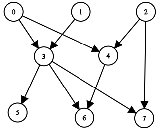
Input: n = 8, edgeList = [[0,3],[0,4],[1,3],[2,4],[2,7],[3,5],[3,6],[3,7],[4,6]]
Output: [[],[],[],[0,1],[0,2],[0,1,3],[0,1,2,3,4],[0,1,2,3]]
Explanation:
The above diagram represents the input graph.
- Nodes 0, 1, and 2 do not have any ancestors.
- Node 3 has two ancestors 0 and 1.
- Node 4 has two ancestors 0 and 2.
- Node 5 has three ancestors 0, 1, and 3.
- Node 6 has five ancestors 0, 1, 2, 3, and 4.
- Node 7 has four ancestors 0, 1, 2, and 3.
Example 2:
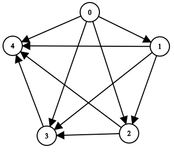
Input: n = 5, edgeList = [[0,1],[0,2],[0,3],[0,4],[1,2],[1,3],[1,4],[2,3],[2,4],[3,4]]
Output: [[],[0],[0,1],[0,1,2],[0,1,2,3]]
Explanation:
The above diagram represents the input graph.
- Node 0 does not have any ancestor.
- Node 1 has one ancestor 0.
- Node 2 has two ancestors 0 and 1.
- Node 3 has three ancestors 0, 1, and 2.
- Node 4 has four ancestors 0, 1, 2, and 3.
Constraints:
1 <= n <= 10000 <= edges.length <= min(2000, n * (n - 1) / 2)edges[i].length == 20 <= fromi, toi <= n - 1fromi != toi- There are no duplicate edges.
- The graph is directed and acyclic.
Approach Overview
Problem Overview: You are given a directed acyclic graph (DAG) with n nodes and edges [u, v]. For every node v, compute all nodes that can reach v. The result must list ancestors for each node in sorted order.
Approach 1: DFS with Topological Sorting (O(n*(n+m)) time, O(n^2) space)
This approach processes the DAG in topological order so every node is visited only after its prerequisites. Build an adjacency list and compute a topological order using topological sort. Maintain a set of ancestors for each node. When processing an edge u -> v, add u to v's ancestor set and union all ancestors of u into v. Because the graph is acyclic, ancestors propagate forward without needing revisits. This method leverages the dependency ordering of DAGs and works well when you already compute topological order.
Approach 2: Reverse Edge DFS (O(n*(n+m)) time, O(n+m) space)
Instead of propagating ancestors forward, flip the edges and search backward. Build a reversed adjacency list where v -> u means u is a parent of v. For every node i, run a depth-first search or breadth-first search on the reversed graph to find all reachable nodes. Those reachable nodes are exactly the ancestors of i. Track visited nodes to avoid cycles (even though DAG guarantees none) and collect results. This approach is conceptually simpler because each search directly discovers the ancestor set for one node.
Recommended for interviews: The topological propagation approach is typically preferred. It demonstrates understanding of DAG processing and avoids repeating full traversals for each node. Reverse DFS still works and is easier to reason about, but interviewers usually expect a solution that leverages topological ordering to propagate ancestor information efficiently across the graph.
Approach 1: DFS and Topological Sorting
This approach involves the following steps:
- Create an adjacency list to represent the graph.
- Perform topological sorting using a DFS to establish the processing order of each node.
- For each node, use the established order to determine its ancestors by propagating the ancestors list from predecessors to successors in the order of DFS completion.
- Finally, sort the ancestors list for each node as required in ascending order.
This solution uses a DFS-based topological sort to process each node in a DAG. We represent the graph as an adjacency list and maintain an indegree count. Nodes with no incoming edges are processed first, during which their ancestors are propagated to their children nodes. This is done until all nodes are processed, yielding a set of ancestors which we then convert to a sorted list for each node to meet the problem requirement.
Complexity
Time Complexity: O(V + E), where V is the number of nodes and E is the number of edges, since we're effectively traversing all nodes and edges.
Space Complexity: O(V + E), due to the storage needed for the graph representation and the ancestors lists.
Approach 2: Reverse Edge DFS
Here, we reverse the edges in the graph and then perform a DFS for each node to find all reachable nodes, which now represent ancestors. This is an implementation that directly finds ancestors by traversing upwards in the graph via reversed edges:
- Create an adjacency list but with reversed edges.
- For each node, perform DFS to locate all nodes that can reach it (which are ancestors in the original graph).
- Cautiously compile and sort results before returning, ensuring a time-efficient DFS exploration by marking visited nodes.
This solution reverses the direction of edges and applies DFS for each node to find reachable nodes (representing ancestors). Each DFS invocation tracks visited nodes to prevent reprocessing and adds ancestors directly to the current node's list, which is then sorted for output.
Complexity
Time Complexity: O(V * (V + E)), due to performing DFS from every node and having potential to traverse the full graph per DFS call.
Space Complexity: O(V + E), where V storage comes from graph information and visited nodes tracking.
Approach 3: BFS
First, we construct the adjacency list g based on the two-dimensional array edges, where g[i] represents all successor nodes of node i.
Then, we enumerate node i as the ancestor node from small to large, use BFS to search all successor nodes of node i, and add node i to the ancestor list of these successor nodes.
The time complexity is O(n^2), and the space complexity is O(n^2). Where n is the number of nodes.
Complexity Comparison
| Approach | Complexity |
|---|---|
| DFS and Topological Sorting | Time Complexity: O(V + E), where V is the number of nodes and E is the number of edges, since we're effectively traversing all nodes and edges. |
| Reverse Edge DFS | Time Complexity: O(V * (V + E)), due to performing DFS from every node and having potential to traverse the full graph per DFS call. |
| BFS | — |
Detailed Complexity Analysis
| Approach | Time | Space | When to Use |
|---|---|---|---|
| DFS with Topological Sort | O(n*(n+m)) | O(n^2) | Best general approach for DAG problems where information propagates along edges |
| Reverse Edge DFS | O(n*(n+m)) | O(n+m) | Simpler logic when computing ancestors independently for each node |
Video Solution
2192. All Ancestors of a Node in a Directed Acyclic Graph || Biweekly Contest 73 || LeetCode 2192 • Bro Coders • 6,453 views views
Watch 9 more video solutions →Frequently Asked Questions
Is All Ancestors of a Node in a Directed Acyclic Graph easy or hard?
All Ancestors of a Node in a Directed Acyclic Graph Python/Java solution
How to solve All Ancestors of a Node in a Directed Acyclic Graph in O(n*(n+m))?
What is the best approach for All Ancestors of a Node in a Directed Acyclic Graph?
Is All Ancestors of a Node in a Directed Acyclic Graph asked at Google/Amazon/Meta?
What data structure is used in All Ancestors of a Node in a Directed Acyclic Graph?
What is the time complexity of All Ancestors of a Node in a Directed Acyclic Graph?
Ready to solve this problem?
Practice All Ancestors of a Node in a Directed Acyclic Graph with our built-in code editor and test cases.
Practice on FleetCode