Given an m x n binary matrix mat, return the distance of the nearest 0 for each cell.
The distance between two cells sharing a common edge is 1.
Example 1:
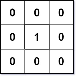
Input: mat = [[0,0,0],[0,1,0],[0,0,0]]
Output: [[0,0,0],[0,1,0],[0,0,0]]
Example 2:
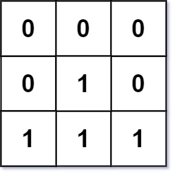
Input: mat = [[0,0,0],[0,1,0],[1,1,1]]
Output: [[0,0,0],[0,1,0],[1,2,1]]
Constraints:
m == mat.lengthn == mat[i].length1 <= m, n <= 1041 <= m * n <= 104mat[i][j] is either 0 or 1.0 in mat.
Note: This question is the same as 1765: https://leetcode.com/problems/map-of-highest-peak/
Problem Overview: You get an m x n binary matrix containing only 0 and 1. For every cell containing 1, compute the distance to the nearest 0. Distance is measured using 4-directional moves (up, down, left, right). The result is another matrix where each cell stores the shortest distance to a zero.
Approach 1: Breadth-First Search (Multi-Source BFS) (Time: O(m*n), Space: O(m*n))
This problem becomes straightforward once you flip the perspective. Instead of starting BFS from every 1, start from every 0 simultaneously. Push all zero cells into a queue and run a multi-source Breadth-First Search. Each expansion updates neighboring cells with distance current + 1. Because BFS explores level by level, the first time a cell is reached guarantees the shortest path to a zero. Use a queue and iterate through the grid once to initialize it. Then repeatedly pop cells, check their four neighbors, and update distances if they haven't been assigned yet. Each cell enters the queue at most once, giving linear time complexity.
This approach works well because BFS naturally computes shortest paths in an unweighted grid. Since all edges have equal cost (1 step), BFS guarantees minimal distance without extra bookkeeping. For grid shortest-path problems involving nearest targets, multi-source BFS is often the cleanest and most interview-friendly pattern. The grid itself can store distances, so only a queue is required for traversal.
Approach 2: Dynamic Programming Two-Pass Scan (Time: O(m*n), Space: O(1) extra)
The same result can be computed using Dynamic Programming with two directional passes. Initialize a distance matrix with a large value for cells containing 1 and 0 for zero cells. First pass: iterate top-left to bottom-right. For each cell, check top and left neighbors and update the distance using min(current, neighbor + 1). Second pass: iterate bottom-right to top-left and check bottom and right neighbors. These two passes propagate the shortest distance information across the grid.
The key insight is that the shortest path to a zero must come from one of the four directions. Splitting the updates into two directional sweeps ensures all possibilities are covered. This method avoids a queue and works purely with iterative updates over the matrix. Time complexity remains linear because each cell is processed a constant number of times.
Recommended for interviews: Multi-source BFS is the approach most interviewers expect. It demonstrates understanding of grid traversal and shortest-path patterns using BFS. The dynamic programming solution is equally optimal but slightly less intuitive unless you already recognize the two-pass DP pattern used in grid distance problems.
The BFS approach involves initializing a queue with all positions of zeros in the matrix, since the distance from any zero to itself is zero. From there, perform a level-order traversal (BFS) to update the distances of the cells that are accessible from these initial zero cells. This approach guarantees that each cell is reached by the shortest path.
In the C implementation, we use a queue to perform a BFS starting from all cells with 0. We then update neighboring cells with the smallest distance possible, propagating the minimum distances to eventually fill out the entire matrix with correct values.
Time Complexity: O(m * n), as each cell is processed at most once.
Space Complexity: O(m * n), for storing the resulting distance matrix and the BFS queue.
The dynamic programming (DP) approach updates the matrix by considering each cell from four possible directions, iterating twice over the matrix to propagate the minimum distances. First, traverse from top-left to bottom-right, and then from bottom-right to top-left, ensuring a comprehensive minimum distance calculation.
In this C code, distance calculation progresses first from the top-left to bottom-right. We then perform a second pass from bottom-right to top-left to integrate the shortest distances possible from alternate directions. The use of INT_MAX - 1 is a sufficient surrogate for infinity.
Time Complexity: O(m * n)
Space Complexity: O(m * n)
We create a matrix ans of the same size as mat and initialize all elements to -1.
Then, we traverse mat, adding the coordinates (i, j) of all 0 elements to the queue q, and setting ans[i][j] to 0.
Next, we use Breadth-First Search (BFS), removing an element (i, j) from the queue and traversing its four directions. If the element in that direction (x, y) satisfies 0 leq x < m, 0 leq y < n and ans[x][y] = -1, then we set ans[x][y] to ans[i][j] + 1 and add (x, y) to the queue q.
Finally, we return ans.
The time complexity is O(m times n), and the space complexity is O(m times n). Here, m and n are the number of rows and columns in the matrix mat, respectively.
| Approach | Complexity |
|---|---|
| Breadth-First Search (BFS) Approach | Time Complexity: O(m * n), as each cell is processed at most once. |
| Dynamic Programming Approach | Time Complexity: O(m * n) |
| BFS | — |
| Approach | Time | Space | When to Use |
|---|---|---|---|
| Multi-Source BFS | O(m*n) | O(m*n) | Best general solution for shortest distance in grids; very intuitive in interviews |
| Dynamic Programming Two-Pass | O(m*n) | O(1) extra | When avoiding queue-based traversal or optimizing memory usage |
Leetcode 542. 01 Matrix - Python • HelmyCodeCamp • 26,077 views views
Watch 9 more video solutions →Practice 01 Matrix with our built-in code editor and test cases.
Practice on FleetCode