There are n cities. Some of them are connected, while some are not. If city a is connected directly with city b, and city b is connected directly with city c, then city a is connected indirectly with city c.
A province is a group of directly or indirectly connected cities and no other cities outside of the group.
You are given an n x n matrix isConnected where isConnected[i][j] = 1 if the ith city and the jth city are directly connected, and isConnected[i][j] = 0 otherwise.
Return the total number of provinces.
Example 1:
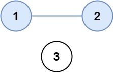
Input: isConnected = [[1,1,0],[1,1,0],[0,0,1]]
Output: 2
Example 2:
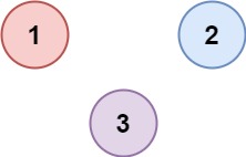
Input: isConnected = [[1,0,0],[0,1,0],[0,0,1]]
Output: 3
Constraints:
1 <= n <= 200n == isConnected.lengthn == isConnected[i].lengthisConnected[i][j] is 1 or 0.isConnected[i][i] == 1isConnected[i][j] == isConnected[j][i]Problem Overview: You are given an n x n adjacency matrix isConnected where isConnected[i][j] = 1 means city i and city j are directly connected. A province is a group of cities connected directly or indirectly. The task is to count how many such provinces exist.
Approach 1: Depth-First Search (DFS) (Time: O(n2), Space: O(n))
Treat the matrix as a graph where each city is a node and isConnected[i][j] = 1 represents an undirected edge. Iterate through every city. When you encounter a city that hasn’t been visited, start a DFS traversal and mark all reachable cities as visited. That traversal covers exactly one connected component, which corresponds to a province. Since the adjacency matrix requires scanning all n neighbors for each node, the traversal costs O(n2). This approach directly applies classic Depth-First Search on a graph and is usually the most intuitive way to reason about connected components.
Approach 2: Union-Find (Disjoint Set) (Time: O(n2 · α(n)), Space: O(n))
Union-Find models each city as part of a disjoint set. Initially every city is its own parent. Scan the adjacency matrix and whenever isConnected[i][j] = 1, perform a union operation to merge the sets containing i and j. Path compression and union-by-rank keep operations nearly constant time, giving an amortized O(α(n)) cost per union. After processing the matrix, the number of unique roots represents the number of provinces. This approach works well when you repeatedly merge components or when connectivity queries appear in larger systems using Union Find.
Recommended for interviews: DFS (or BFS) is the most expected explanation because the problem maps directly to counting connected components in a graph. Interviewers want to see that you recognize the adjacency matrix as a graph representation and run a traversal to mark visited nodes. Union-Find is equally valid and demonstrates deeper familiarity with graph connectivity techniques. Start with DFS to show clear reasoning, then mention Union-Find as an alternative optimization pattern.
This approach uses Depth-First Search (DFS) to count the number of provinces. The core idea is to treat the connected cities as a graph and perform a DFS traversal starting from each city. During traversal, mark all reachable cities from the starting city. Each starting city for a DFS that visits new cities indicates the discovery of a new province.
The objective is to find connected components in the graph, which represent provinces. We declare a boolean array visited to track visited cities. We implement a helper function dfs to perform DFS traversal from each unvisited node, marking all reachable nodes. Each DFS starting from an unvisited node suggests a new province has been found.
Time Complexity: O(n^2), as we may visit each cell in the matrix.
Space Complexity: O(n) for the visited array.
This approach employs the Union-Find (Disjoint Set Union) algorithm to find the number of provinces. This algorithm efficiently handles dynamic connectivity queries. By iteratively checking connections and performing unions, we can identify distinct connected components (provinces).
The Union-Find approach involves two primary operations: 'find' and 'union'. Each city starts as its own component, and each connection adds to the union. The find method returns the root ancestor for any node, which helps in determining connected components. The total provinces are the count of unique roots in the parent array.
Time Complexity: O(n^2 * α(n)), where α is the inverse Ackermann function representing nearly constant time for union-find operations.
Space Complexity: O(n), the space for parent and rank arrays.
| Approach | Complexity |
|---|---|
| Approach 1: Depth-First Search (DFS) | Time Complexity: O(n^2), as we may visit each cell in the matrix. |
| Approach 2: Union-Find | Time Complexity: O(n^2 * α(n)), where α is the inverse Ackermann function representing nearly constant time for union-find operations. |
| Approach | Time | Space | When to Use |
|---|---|---|---|
| Depth-First Search (DFS) | O(n^2) | O(n) | Best general solution when treating the matrix as a graph and counting connected components. |
| Union-Find (Disjoint Set) | O(n^2 · α(n)) | O(n) | Useful when repeatedly merging components or solving dynamic connectivity problems. |
G-7. Number of Provinces | C++ | Java | Connected Components • take U forward • 535,400 views views
Watch 9 more video solutions →Practice Number of Provinces with our built-in code editor and test cases.
Practice on FleetCode