According to Wikipedia's article: "The Game of Life, also known simply as Life, is a cellular automaton devised by the British mathematician John Horton Conway in 1970."
The board is made up of an m x n grid of cells, where each cell has an initial state: live (represented by a 1) or dead (represented by a 0). Each cell interacts with its eight neighbors (horizontal, vertical, diagonal) using the following four rules (taken from the above Wikipedia article):
The next state of the board is determined by applying the above rules simultaneously to every cell in the current state of the m x n grid board. In this process, births and deaths occur simultaneously.
Given the current state of the board, update the board to reflect its next state.
Note that you do not need to return anything.
Example 1:
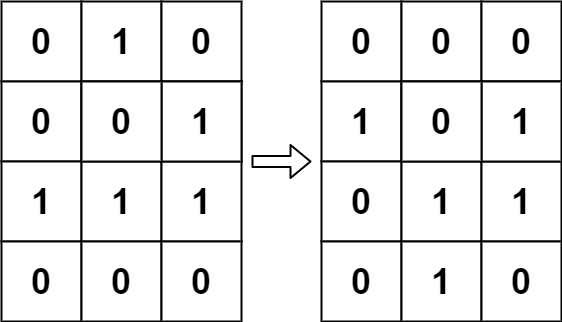
Input: board = [[0,1,0],[0,0,1],[1,1,1],[0,0,0]]
Output: [[0,0,0],[1,0,1],[0,1,1],[0,1,0]]
Example 2:
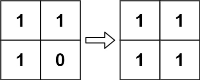
Input: board = [[1,1],[1,0]]
Output: [[1,1],[1,1]]
Constraints:
m == board.lengthn == board[i].length1 <= m, n <= 25board[i][j] is 0 or 1.
Follow up:
Problem Overview: You are given an m x n grid representing Conway’s Game of Life where each cell is either alive (1) or dead (0). Every cell updates simultaneously based on the number of live neighbors among the eight surrounding cells. The challenge is computing the next state of the board without corrupting neighbor calculations while you iterate through the grid.
Approach 1: Naive Approach with Extra Space (O(m*n) time, O(m*n) space)
Iterate through the grid and count the eight neighbors for each cell. Instead of updating the board immediately, store the next state in a separate m x n matrix. For each cell: if it is alive and has fewer than 2 or more than 3 live neighbors, it dies; if it has exactly 2 or 3 neighbors, it survives; a dead cell with exactly 3 neighbors becomes alive. After processing every cell, copy the new matrix back into the original board. This approach is straightforward and mirrors the rules directly, making it useful when clarity matters more than memory efficiency.
The main downside is the extra memory allocation. The algorithm still touches each cell once and checks up to eight neighbors, so the time complexity remains O(m*n). Space complexity is also O(m*n) due to the additional board. Problems like this commonly appear in array and matrix traversal scenarios where state must not be overwritten during iteration.
Approach 2: In-Place State Transition (O(m*n) time, O(1) space)
The optimal solution modifies the board in-place by encoding both the old and new states inside the same cell. While scanning the grid, mark transitional states instead of immediately overwriting values. A common encoding strategy uses:
-1 for a cell that was alive but becomes dead, and 2 for a cell that was dead but becomes alive. When counting neighbors, treat values 1 and -1 as originally alive because they represent cells that were alive before the update.
First pass: iterate through the grid, count neighbors, and assign transitional markers according to the Game of Life rules. Second pass: normalize the board by converting all positive values to 1 and all others to 0. Because transitional values preserve the previous state, neighbor counts remain correct even after partial updates.
This technique is a classic simulation pattern where temporary state encoding avoids extra memory. The board is still processed once, giving O(m*n) time complexity, while space complexity drops to O(1).
Recommended for interviews: Interviewers typically expect the in-place transition approach. The extra-space version demonstrates you understand the Game of Life rules and grid traversal, but the in-place encoding shows stronger problem-solving skills and awareness of memory optimization patterns commonly used in matrix simulations.
This approach creates a copy of the original board. It calculates the new state for each cell using the current state from the original board while updating the new state in the copy. Once all cells have been processed, it updates the original board with the calculated states from the copy.
This C solution uses an additional matrix to store the new state of each cell while retaining the current state in the original matrix. For each cell, its live neighbors are counted, and rules are applied to determine its next state. Once every cell's state is determined, the original board is updated. Memory is dynamically allocated for the copy and freed after use.
Time Complexity: O(m * n), where m is the number of rows and n is the number of columns, because each cell is visited once.
Space Complexity: O(m * n), due to the additional copy of the board.
This approach uses in-place updates by leveraging different state values. We introduce temporary states: 2 represents a cell that was originally live (1) but will be dead in the next state, and -1 represents a cell that was dead (0) but will be live in the next state. At the end, these temporary states are converted to the final states.
The C solution uses the board itself to track changes by representing transitional states so the board can be accurately updated in one iteration by determining the final state in a second pass.
Time Complexity: O(m * n), where m is the number of rows and n is the number of columns.
Space Complexity: O(1), as no additional space is used beyond input storage.
Let's define two new states. State 2 indicates that the living cell becomes dead in the next state, and state -1 indicates that the dead cell becomes alive in the next state. Therefore, for the current grid we are traversing, if the grid is greater than 0, it means that the current grid is a living cell, otherwise it is a dead cell.
So we can traverse the entire board, for each grid, count the number of living neighbors around the grid, and use the variable live to represent it. If the current grid is a living cell, then when live \lt 2 or live \gt 3, the next state of the current grid is a dead cell, that is, state 2; if the current grid is a dead cell, then when live = 3, the next state of the current grid is an active cell, that is, state -1.
Finally, we traverse the board again, and update the grid with state 2 to a dead cell, and update the grid with state -1 to an active cell.
The time complexity is O(m times n), where m and n are the number of rows and columns of the board, respectively. We need to traverse the entire board. And the space complexity is O(1).
| Approach | Complexity |
|---|---|
| Naive Approach with Extra Space | Time Complexity: O(m * n), where m is the number of rows and n is the number of columns, because each cell is visited once. |
| In-Place State Transition Approach | Time Complexity: O(m * n), where m is the number of rows and n is the number of columns. |
| In-place marking | — |
| Approach | Time | Space | When to Use |
|---|---|---|---|
| Naive Approach with Extra Space | O(m*n) | O(m*n) | Best for clarity and quick implementation when memory usage is not constrained |
| In-Place State Transition | O(m*n) | O(1) | Preferred in interviews and production when memory efficiency matters |
Game of Life - Leetcode 289 - Python • NeetCode • 58,595 views views
Watch 9 more video solutions →Practice Game of Life with our built-in code editor and test cases.
Practice on FleetCodePractice this problem
Open in Editor