Watch 10 video solutions for Sparse Matrix Multiplication, a medium level problem involving Array, Hash Table, Matrix. This walkthrough by Happy Coding has 12,502 views views. Want to try solving it yourself? Practice on FleetCode or read the detailed text solution.
Given two sparse matrices mat1 of size m x k and mat2 of size k x n, return the result of mat1 x mat2. You may assume that multiplication is always possible.
Example 1:
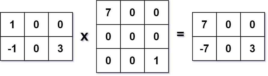
Input: mat1 = [[1,0,0],[-1,0,3]], mat2 = [[7,0,0],[0,0,0],[0,0,1]]
Output: [[7,0,0],[-7,0,3]]
Example 2:
Input: mat1 = [[0]], mat2 = [[0]]
Output: [[0]]
Constraints:
m == mat1.lengthk == mat1[i].length == mat2.lengthn == mat2[i].length1 <= m, n, k <= 100-100 <= mat1[i][j], mat2[i][j] <= 100Problem Overview: You are given two matrices mat1 and mat2. The task is to compute their matrix product. The twist is that the matrices are sparse, meaning most values are zero. A good solution avoids unnecessary multiplications with zero.
Approach 1: Direct Multiplication (O(m * n * p) time, O(1) extra space)
This approach follows the standard matrix multiplication rule. For each cell result[i][j], iterate through index k and compute mat1[i][k] * mat2[k][j]. The key optimization is skipping work when mat1[i][k] == 0, because multiplying by zero contributes nothing to the result. Implementation uses three nested loops over rows of mat1, columns of mat2, and the shared dimension. Even with the zero check, the worst‑case complexity remains O(m * n * p) where m, n, and p are the matrix dimensions. This approach is simple and readable but wastes time when matrices contain many zeros. It mainly relies on basic Array iteration and standard Matrix multiplication rules.
Approach 2: Preprocessing Non‑Zero Values (O(nnz(A) * p) average time, O(nnz(A) + nnz(B)) space)
Sparse matrices benefit from processing only non‑zero entries. First preprocess mat1 and record the column indices and values of non‑zero elements for every row. This structure can be stored using lists or a Hash Table. During multiplication, iterate through the stored non‑zero elements (i, k) from mat1. For each one, multiply it with the corresponding row k in mat2. Since the multiplication happens only when mat1[i][k] is non‑zero, the algorithm skips most useless operations. The runtime becomes proportional to the number of non‑zero values rather than the total matrix size. If nnz(A) is the number of non‑zero entries in mat1, the effective work is roughly O(nnz(A) * p) or better depending on sparsity in mat2. Extra space stores the non‑zero structure, but the speed improvement is significant for large sparse matrices.
Recommended for interviews: Interviewers expect the preprocessing approach. Starting with direct multiplication shows you understand matrix multiplication basics, but recognizing sparsity and skipping zero work demonstrates stronger algorithmic thinking. Mention the idea of storing only non‑zero elements and multiplying selectively. That insight turns a brute force triple loop into a solution that scales with the actual useful data rather than the full matrix size.
| Approach | Time | Space | When to Use |
|---|---|---|---|
| Direct Multiplication | O(m * n * p) | O(1) | Small matrices or when sparsity is low and implementation simplicity matters |
| Direct Multiplication with Zero Skip | O(m * n * p) worst case | O(1) | Slight optimization when many values in the first matrix are zero |
| Preprocessing Non‑Zero Values | ~O(nnz(A) * p) | O(nnz(A) + nnz(B)) | Large sparse matrices where skipping zero operations drastically reduces work |