Watch 10 video solutions for Number of Islands II, a hard level problem involving Array, Hash Table, Union Find. This walkthrough by Ren Zhang has 7,287 views views. Want to try solving it yourself? Practice on FleetCode or read the detailed text solution.
You are given an empty 2D binary grid grid of size m x n. The grid represents a map where 0's represent water and 1's represent land. Initially, all the cells of grid are water cells (i.e., all the cells are 0's).
We may perform an add land operation which turns the water at position into a land. You are given an array positions where positions[i] = [ri, ci] is the position (ri, ci) at which we should operate the ith operation.
Return an array of integers answer where answer[i] is the number of islands after turning the cell (ri, ci) into a land.
An island is surrounded by water and is formed by connecting adjacent lands horizontally or vertically. You may assume all four edges of the grid are all surrounded by water.
Example 1:
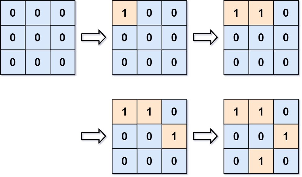
Input: m = 3, n = 3, positions = [[0,0],[0,1],[1,2],[2,1]]
Output: [1,1,2,3]
Explanation:
Initially, the 2d grid is filled with water.
- Operation #1: addLand(0, 0) turns the water at grid[0][0] into a land. We have 1 island.
- Operation #2: addLand(0, 1) turns the water at grid[0][1] into a land. We still have 1 island.
- Operation #3: addLand(1, 2) turns the water at grid[1][2] into a land. We have 2 islands.
- Operation #4: addLand(2, 1) turns the water at grid[2][1] into a land. We have 3 islands.
Example 2:
Input: m = 1, n = 1, positions = [[0,0]]
Output: [1]
Constraints:
1 <= m, n, positions.length <= 1041 <= m * n <= 104positions[i].length == 20 <= ri < m0 <= ci < n
Follow up: Could you solve it in time complexity O(k log(mn)), where k == positions.length?
Problem Overview: You start with an empty m x n water grid. Land positions are added one by one. After each addition, return the current number of islands. The challenge is updating the island count efficiently as the grid evolves.
Approach 1: Recompute Islands with DFS/BFS (O(k * m * n) time, O(m * n) space)
After every land addition, rebuild the entire island count by scanning the grid and running DFS or BFS from each unvisited land cell. This uses a standard flood-fill traversal across the grid stored in an array. The approach is simple but extremely expensive because you reprocess the whole grid for each operation. With k additions, the complexity becomes O(k * m * n), which quickly times out for large grids.
Approach 2: Incremental BFS Merge (O(k * m * n) worst-case time, O(m * n) space)
Instead of recomputing everything, treat each new land cell as a new island and then check its four neighbors. If neighboring cells already belong to islands, run a traversal to merge connected components. A hash table or grid structure tracks visited cells and island IDs. This avoids scanning the entire grid each time, but merges can still trigger large traversals. In dense grids, repeated BFS/DFS merges degrade back to near O(k * m * n).
Approach 3: Union-Find (Disjoint Set Union) (O(k α(mn)) time, O(m * n) space)
Union-Find models the grid as a set of disjoint components. Each cell maps to a unique index. When you add land, initialize a new set and increase the island count. Check the four neighboring cells; if any neighbor is already land, union their sets. If two previously separate components merge, decrement the island count. Path compression and union by rank make operations nearly constant time, giving an overall complexity of O(k α(mn)), where α is the inverse Ackermann function. This approach relies on the Union Find data structure to efficiently maintain connected components as the grid updates.
Recommended for interviews: Union-Find is the expected solution. Interviewers want to see that you recognize the dynamic connectivity pattern and model islands as disjoint sets. Explaining the brute-force DFS approach first shows baseline understanding, but implementing Union-Find demonstrates strong algorithmic skill and familiarity with near-constant-time connectivity operations.
| Approach | Time | Space | When to Use |
|---|---|---|---|
| Recompute with DFS/BFS | O(k * m * n) | O(m * n) | Conceptual baseline or very small grids |
| Incremental BFS Merge | O(k * m * n) worst case | O(m * n) | When experimenting with dynamic merges without DSU |
| Union-Find (Disjoint Set) | O(k α(mn)) | O(m * n) | Optimal solution for dynamic connectivity problems |