Watch 10 video solutions for Minimum Path Sum, a medium level problem involving Array, Dynamic Programming, Matrix. This walkthrough by Techdose has 88,692 views views. Want to try solving it yourself? Practice on FleetCode or read the detailed text solution.
Given a m x n grid filled with non-negative numbers, find a path from top left to bottom right, which minimizes the sum of all numbers along its path.
Note: You can only move either down or right at any point in time.
Example 1:
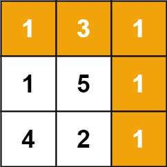
Input: grid = [[1,3,1],[1,5,1],[4,2,1]]
Output: 7
Explanation: Because the path 1 → 3 → 1 → 1 → 1 minimizes the sum.
Example 2:
Input: grid = [[1,2,3],[4,5,6]]
Output: 12
Constraints:
m == grid.lengthn == grid[i].length1 <= m, n <= 2000 <= grid[i][j] <= 200Problem Overview: You are given an m x n grid filled with non‑negative numbers. Starting at the top-left cell, move only right or down until reaching the bottom-right cell. The goal is to compute the minimum possible sum of all values along the path.
Approach 1: Recursive Exploration (Exponential Time)
The most straightforward idea is to explore every possible path using recursion. From any cell (i, j), you have two choices: move right to (i, j+1) or down to (i+1, j). Recursively compute the path sum for both directions and take the minimum. This works but recomputes the same subproblems many times. The time complexity becomes O(2^(m+n)) with O(m+n) recursion stack space, which quickly becomes infeasible for larger grids.
Approach 2: Dynamic Programming with Extra Space (O(m*n) time, O(m*n) space)
Dynamic programming removes repeated computation by storing results for each cell. Create a DP table where dp[i][j] represents the minimum cost to reach cell (i, j). Each cell depends only on the top and left neighbors, so the recurrence becomes dp[i][j] = grid[i][j] + min(dp[i-1][j], dp[i][j-1]). Initialize the first row and first column because they have only one possible direction of movement. Iterate through the grid row by row to fill the table. This approach processes each cell exactly once, giving O(m*n) time and O(m*n) space.
Approach 3: Dynamic Programming with In-Place Modification (O(m*n) time, O(1) extra space)
The DP table is not strictly necessary because the grid itself can store the cumulative minimum cost. Start by updating the first row and first column with running sums since there is only one way to reach those cells. For the remaining cells, update the value using the same recurrence: grid[i][j] += min(grid[i-1][j], grid[i][j-1]). By the time you reach the bottom-right corner, it holds the minimum path sum. This approach still runs in O(m*n) time but reduces auxiliary space to O(1) since the input grid stores the DP state.
Problems like this are classic examples of grid-based dynamic programming. Each state depends on previously computed states in a structured traversal. The grid structure also makes it closely related to matrix traversal problems and common array DP patterns.
Recommended for interviews: Interviewers expect the dynamic programming solution. Starting with the recursive idea demonstrates understanding of the search space, but quickly optimizing it with DP shows you recognize overlapping subproblems. The in-place DP variant is typically considered the most polished solution because it achieves optimal O(m*n) time while keeping extra space at O(1).
| Approach | Time | Space | When to Use |
|---|---|---|---|
| Recursive Exploration | O(2^(m+n)) | O(m+n) | Conceptual starting point to understand all possible paths |
| Dynamic Programming (Extra 2D Table) | O(m*n) | O(m*n) | Clear and easy implementation when modifying the input grid is not allowed |
| Dynamic Programming (In-Place Grid Update) | O(m*n) | O(1) | Optimal interview solution when the grid can be reused to store DP values |