Watch 10 video solutions for Minimum Falling Path Sum, a medium level problem involving Array, Dynamic Programming, Matrix. This walkthrough by codestorywithMIK has 17,212 views views. Want to try solving it yourself? Practice on FleetCode or read the detailed text solution.
Given an n x n array of integers matrix, return the minimum sum of any falling path through matrix.
A falling path starts at any element in the first row and chooses the element in the next row that is either directly below or diagonally left/right. Specifically, the next element from position (row, col) will be (row + 1, col - 1), (row + 1, col), or (row + 1, col + 1).
Example 1:
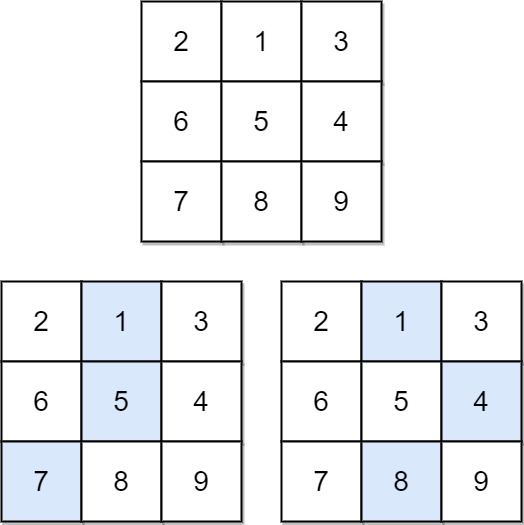
Input: matrix = [[2,1,3],[6,5,4],[7,8,9]]
Output: 13
Explanation: There are two falling paths with a minimum sum as shown.
Example 2:
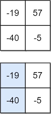
Input: matrix = [[-19,57],[-40,-5]]
Output: -59
Explanation: The falling path with a minimum sum is shown.
Constraints:
n == matrix.length == matrix[i].length1 <= n <= 100-100 <= matrix[i][j] <= 100Problem Overview: You are given an n x n matrix of integers. A falling path starts at any cell in the first row and moves to the next row either directly below, diagonally left, or diagonally right. The goal is to compute the minimum possible sum of values along any valid falling path from the top row to the bottom row.
Approach 1: Top-Down Dynamic Programming with Memoization (Time: O(n^2), Space: O(n^2))
This approach models the problem as recursion over rows. For each cell (r, c), recursively compute the minimum path sum starting from that cell by exploring the three valid next positions: (r+1, c-1), (r+1, c), and (r+1, c+1). Many subproblems repeat, so store results in a memo table to avoid recomputation. Each cell is solved once, which reduces exponential recursion to quadratic time. This method is intuitive if you think in terms of exploring all paths but caching results.
The recursion stops when the last row is reached. Out-of-bound column moves are ignored. Because every matrix cell is computed once and stored, the complexity becomes O(n^2). This pattern is common in dynamic programming problems on grids.
Approach 2: Bottom-Up Dynamic Programming (Time: O(n^2), Space: O(n^2) or O(1) in-place)
The bottom-up strategy processes the matrix row by row. Starting from the second row, update each cell by adding the minimum of the three reachable cells from the previous row: up-left, up, and up-right. This converts the matrix into a DP table where each entry represents the minimum path sum reaching that cell.
For cell (r, c), compute matrix[r][c] += min(prev[c], prev[c-1], prev[c+1]) while handling boundary columns carefully. After processing all rows, the answer is the minimum value in the last row. This method iterates once over the grid and avoids recursion overhead. Because the DP values can overwrite the original matrix, the extra space can be reduced to O(1).
This technique is typical for problems involving transitions in a matrix or grid where each state depends on nearby cells. Iterating through the array structure row by row keeps the implementation simple and efficient.
Recommended for interviews: Bottom-up dynamic programming is the expected solution. It demonstrates that you can convert recursive state transitions into iterative DP and optimize space if needed. Showing the top-down memoized version first can help explain the recurrence, but the bottom-up implementation signals stronger DP problem-solving skills.
| Approach | Time | Space | When to Use |
|---|---|---|---|
| Top-Down DP with Memoization | O(n^2) | O(n^2) | When deriving the recurrence relation or explaining the problem using recursion |
| Bottom-Up Dynamic Programming | O(n^2) | O(n^2) or O(1) in-place | Preferred for production or interviews due to iterative structure and possible space optimization |