Watch 2 video solutions for Minimum Cost to Buy Apples, a medium level problem involving Array, Graph, Heap (Priority Queue). This walkthrough by Programming Live with Larry has 612 views views. Want to try solving it yourself? Practice on FleetCode or read the detailed text solution.
You are given a positive integer n representing n cities numbered from 1 to n. You are also given a 2D array roads, where roads[i] = [ai, bi, costi] indicates that there is a bidirectional road between cities ai and bi with a cost of traveling equal to costi.
You can buy apples in any city you want, but some cities have different costs to buy apples. You are given the 1-based array appleCost where appleCost[i] is the cost of buying one apple from city i.
You start at some city, traverse through various roads, and eventually buy exactly one apple from any city. After you buy that apple, you have to return back to the city you started at, but now the cost of all the roads will be multiplied by a given factor k.
Given the integer k, return a 1-based array answer of size n where answer[i] is the minimum total cost to buy an apple if you start at city i.
Example 1:
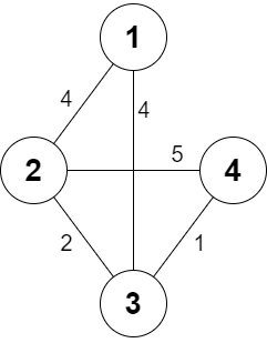
Input: n = 4, roads = [[1,2,4],[2,3,2],[2,4,5],[3,4,1],[1,3,4]], appleCost = [56,42,102,301], k = 2
Output: [54,42,48,51]
Explanation: The minimum cost for each starting city is the following:
- Starting at city 1: You take the path 1 -> 2, buy an apple at city 2, and finally take the path 2 -> 1. The total cost is 4 + 42 + 4 * 2 = 54.
- Starting at city 2: You directly buy an apple at city 2. The total cost is 42.
- Starting at city 3: You take the path 3 -> 2, buy an apple at city 2, and finally take the path 2 -> 3. The total cost is 2 + 42 + 2 * 2 = 48.
- Starting at city 4: You take the path 4 -> 3 -> 2 then you buy at city 2, and finally take the path 2 -> 3 -> 4. The total cost is 1 + 2 + 42 + 1 * 2 + 2 * 2 = 51.
Example 2:
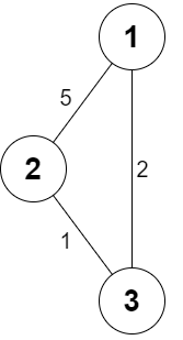
Input: n = 3, roads = [[1,2,5],[2,3,1],[3,1,2]], appleCost = [2,3,1], k = 3
Output: [2,3,1]
Explanation: It is always optimal to buy the apple in the starting city.
Constraints:
2 <= n <= 10001 <= roads.length <= 20001 <= ai, bi <= nai != bi1 <= costi <= 105appleCost.length == n1 <= appleCost[i] <= 1051 <= k <= 100Problem Overview: You have n cities connected by weighted roads. Each city sells apples at a specific price. Starting from city i, you can travel to any city j to buy apples and return back. The return trip multiplies road cost by k. For every city, compute the minimum total cost of buying apples and coming back.
Approach 1: Run Dijkstra from Every City (Brute Force Graph Shortest Path) (Time: O(n * (m log n)), Space: O(n))
Treat each city as a starting point. Run Dijkstra to compute the shortest distance from city i to every other city. For each destination j, calculate the purchase cost appleCost[j] + dist(i, j) * (k + 1). Track the minimum value. This works because traveling to j and returning multiplies each road cost by (k + 1). The downside is obvious: running a full shortest-path search for every city is expensive when n is large.
Approach 2: Multi‑Source Dijkstra with Heap Optimization (Time: O((n + m) log n), Space: O(n))
The key insight: the cost formula appleCost[j] + (k + 1) * dist(i, j) can be interpreted as a shortest-path problem starting from all apple cities simultaneously. Initialize a priority queue with every city j using distance appleCost[j]. When relaxing edges, scale each road weight by (k + 1). Running a single shortest path search propagates the cheapest apple purchase cost to every city. The heap (priority queue) always expands the currently cheapest state, just like standard graph Dijkstra.
This transforms the problem into a classic multi‑source shortest path. Instead of asking "where should city i go to buy apples", the algorithm spreads the apple prices outward across the graph with adjusted edge weights.
Recommended for interviews: The heap‑optimized multi‑source Dijkstra approach. Interviewers expect you to recognize the shortest‑path structure and reduce repeated computations. Explaining the brute‑force per‑city Dijkstra first shows baseline reasoning, while the multi‑source optimization demonstrates strong graph intuition.
| Approach | Time | Space | When to Use |
|---|---|---|---|
| Run Dijkstra from Every City | O(n * (m log n)) | O(n) | Small graphs where repeated shortest-path runs are acceptable |
| Multi-Source Heap-Optimized Dijkstra | O((n + m) log n) | O(n) | General case and optimal solution for large graphs |