Watch 6 video solutions for Maximize Grid Happiness, a hard level problem involving Dynamic Programming, Bit Manipulation, Memoization. This walkthrough by Hua Hua has 2,614 views views. Want to try solving it yourself? Practice on FleetCode or read the detailed text solution.
You are given four integers, m, n, introvertsCount, and extrovertsCount. You have an m x n grid, and there are two types of people: introverts and extroverts. There are introvertsCount introverts and extrovertsCount extroverts.
You should decide how many people you want to live in the grid and assign each of them one grid cell. Note that you do not have to have all the people living in the grid.
The happiness of each person is calculated as follows:
120 happiness and lose 30 happiness for each neighbor (introvert or extrovert).40 happiness and gain 20 happiness for each neighbor (introvert or extrovert).Neighbors live in the directly adjacent cells north, east, south, and west of a person's cell.
The grid happiness is the sum of each person's happiness. Return the maximum possible grid happiness.
Example 1:
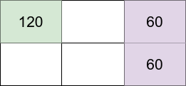
Input: m = 2, n = 3, introvertsCount = 1, extrovertsCount = 2
Output: 240
Explanation: Assume the grid is 1-indexed with coordinates (row, column).
We can put the introvert in cell (1,1) and put the extroverts in cells (1,3) and (2,3).
- Introvert at (1,1) happiness: 120 (starting happiness) - (0 * 30) (0 neighbors) = 120
- Extrovert at (1,3) happiness: 40 (starting happiness) + (1 * 20) (1 neighbor) = 60
- Extrovert at (2,3) happiness: 40 (starting happiness) + (1 * 20) (1 neighbor) = 60
The grid happiness is 120 + 60 + 60 = 240.
The above figure shows the grid in this example with each person's happiness. The introvert stays in the light green cell while the extroverts live on the light purple cells.
Example 2:
Input: m = 3, n = 1, introvertsCount = 2, extrovertsCount = 1
Output: 260
Explanation: Place the two introverts in (1,1) and (3,1) and the extrovert at (2,1).
- Introvert at (1,1) happiness: 120 (starting happiness) - (1 * 30) (1 neighbor) = 90
- Extrovert at (2,1) happiness: 40 (starting happiness) + (2 * 20) (2 neighbors) = 80
- Introvert at (3,1) happiness: 120 (starting happiness) - (1 * 30) (1 neighbor) = 90
The grid happiness is 90 + 80 + 90 = 260.
Example 3:
Input: m = 2, n = 2, introvertsCount = 4, extrovertsCount = 0
Output: 240
Constraints:
1 <= m, n <= 50 <= introvertsCount, extrovertsCount <= min(m * n, 6)Problem Overview: You are given an m x n grid and a limited number of introverts and extroverts. Each person contributes a base happiness value, but neighboring cells change that value depending on the combination of people placed. The goal is to place people in the grid so the total happiness score is maximized.
Approach 1: Backtracking with Pruning (Exponential Time, O(3^(m*n)) time, O(m*n) space)
This approach explores every possible way to fill the grid: leave the cell empty, place an introvert, or place an extrovert. During recursion you track remaining introverts/extroverts and compute the incremental happiness contribution from the top and left neighbors. Pruning helps reduce work by stopping branches where remaining cells cannot beat the current best score. While conceptually straightforward, the branching factor of three per cell leads to exponential complexity, so it only works because the grid size is small. This method is useful for understanding the scoring mechanics before introducing dynamic programming.
Approach 2: Dynamic Programming with State Representation (O(m * 3^n * 3^n * introverts * extroverts) time, O(3^n * introverts * extroverts) space)
The optimal solution compresses each row configuration into a base‑3 state where each cell is 0 = empty, 1 = introvert, or 2 = extrovert. Since n ≤ 5, there are at most 3^5 = 243 possible row states. Precompute three things for every state: how many introverts/extroverts it uses, the internal row happiness, and the interaction score with another row above it. Then run DP row by row where the state is dp[row][prevState][introvertsLeft][extrovertsLeft]. For each row you iterate over all valid current states and combine them with the previous row state. This captures both horizontal and vertical neighbor effects while dramatically reducing the search space. The state compression technique is a classic combination of bitmask/state encoding and memoization to reuse overlapping subproblems.
Recommended for interviews: The dynamic programming state‑compression approach is what interviewers expect. Backtracking shows you understand the constraints and happiness rules, but it scales poorly. The DP solution demonstrates stronger problem‑solving skills: recognizing small grid width, encoding row states efficiently, and reusing results with memoization.
| Approach | Time | Space | When to Use |
|---|---|---|---|
| Backtracking with Pruning | O(3^(m*n)) | O(m*n) | Good for understanding the scoring rules and brute-force reasoning on very small grids. |
| Dynamic Programming with Row State Compression | O(m * 3^n * 3^n * I * E) | O(3^n * I * E) | Optimal approach when grid width is small (n ≤ 5). Efficiently handles neighbor interactions using precomputed row states. |