Watch 10 video solutions for Design Graph With Shortest Path Calculator, a hard level problem involving Graph, Design, Heap (Priority Queue). This walkthrough by codestorywithMIK has 5,468 views views. Want to try solving it yourself? Practice on FleetCode or read the detailed text solution.
There is a directed weighted graph that consists of n nodes numbered from 0 to n - 1. The edges of the graph are initially represented by the given array edges where edges[i] = [fromi, toi, edgeCosti] meaning that there is an edge from fromi to toi with the cost edgeCosti.
Implement the Graph class:
Graph(int n, int[][] edges) initializes the object with n nodes and the given edges.addEdge(int[] edge) adds an edge to the list of edges where edge = [from, to, edgeCost]. It is guaranteed that there is no edge between the two nodes before adding this one.int shortestPath(int node1, int node2) returns the minimum cost of a path from node1 to node2. If no path exists, return -1. The cost of a path is the sum of the costs of the edges in the path.
Example 1:
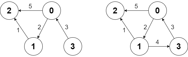
Input
["Graph", "shortestPath", "shortestPath", "addEdge", "shortestPath"]
[[4, [[0, 2, 5], [0, 1, 2], [1, 2, 1], [3, 0, 3]]], [3, 2], [0, 3], [[1, 3, 4]], [0, 3]]
Output
[null, 6, -1, null, 6]

Explanation
Graph g = new Graph(4, [[0, 2, 5], [0, 1, 2], [1, 2, 1], [3, 0, 3]]);
g.shortestPath(3, 2); // return 6. The shortest path from 3 to 2 in the first diagram above is 3 -> 0 -> 1 -> 2 with a total cost of 3 + 2 + 1 = 6.
g.shortestPath(0, 3); // return -1. There is no path from 0 to 3.
g.addEdge([1, 3, 4]); // We add an edge from node 1 to node 3, and we get the second diagram above.
g.shortestPath(0, 3); // return 6. The shortest path from 0 to 3 now is 0 -> 1 -> 3 with a total cost of 2 + 4 = 6.
Constraints:
1 <= n <= 1000 <= edges.length <= n * (n - 1)edges[i].length == edge.length == 30 <= fromi, toi, from, to, node1, node2 <= n - 11 <= edgeCosti, edgeCost <= 106100 calls will be made for addEdge.100 calls will be made for shortestPath.Problem Overview: You need to design a graph data structure that supports two operations: dynamically adding directed weighted edges and computing the shortest path between two nodes. The challenge is balancing update time (addEdge) with query time (shortestPath) while keeping the structure efficient for multiple operations.
Approach 1: Dijkstra's Algorithm with Adjacency List (Time: O((V + E) log V) per query, Space: O(V + E))
Store the graph using an adjacency list where each node keeps a list of (neighbor, weight) pairs. When addEdge is called, append the edge directly to the adjacency list in O(1) time. For shortestPath, run Dijkstra’s algorithm starting from the source node using a min-heap (priority queue). The heap always expands the node with the smallest known distance, ensuring optimal paths in graphs with non‑negative weights. This approach works well when edge additions are frequent but shortest-path queries are moderate. It relies heavily on a heap (priority queue) and classic graph traversal techniques.
Approach 2: Floyd–Warshall Algorithm with Distance Matrix (Time: O(V^3) preprocessing, O(1) query, Space: O(V^2))
Maintain a 2D matrix dist[i][j] representing the shortest distance between every pair of nodes. During initialization, run the Floyd–Warshall algorithm to compute all-pairs shortest paths. Each shortestPath query then becomes a constant-time lookup. When addEdge is called, update the matrix by relaxing paths that could improve using the new edge (u → v). Specifically, iterate over all node pairs and check if going through the new edge shortens their route. This method uses dynamic programming over a shortest path matrix and is ideal when the graph has relatively small n but many queries.
Recommended for interviews: Dijkstra’s algorithm is usually the expected answer. It keeps the design simple, handles dynamic edge additions naturally, and avoids the heavy O(V^3) preprocessing cost. Mentioning Floyd–Warshall shows deeper understanding of all‑pairs shortest path strategies and tradeoffs between preprocessing and query speed.
| Approach | Time | Space | When to Use |
|---|---|---|---|
| Dijkstra with Adjacency List | O((V + E) log V) per query | O(V + E) | General case with dynamic edge additions and moderate query count |
| Floyd–Warshall with Distance Matrix | O(V^3) preprocessing, O(1) query | O(V^2) | Small graphs with many shortest-path queries where constant-time lookup is valuable |