Watch 3 video solutions for Construct 2D Grid Matching Graph Layout, a hard level problem involving Array, Hash Table, Graph. This walkthrough by CodeFod has 820 views views. Want to try solving it yourself? Practice on FleetCode or read the detailed text solution.
You are given a 2D integer array edges representing an undirected graph having n nodes, where edges[i] = [ui, vi] denotes an edge between nodes ui and vi.
Construct a 2D grid that satisfies these conditions:
0 to n - 1 in its cells, with each node appearing exactly once.edges.It is guaranteed that edges can form a 2D grid that satisfies the conditions.
Return a 2D integer array satisfying the conditions above. If there are multiple solutions, return any of them.
Example 1:
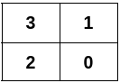
Input: n = 4, edges = [[0,1],[0,2],[1,3],[2,3]]
Output: [[3,1],[2,0]]
Explanation:
Example 2:
Input: n = 5, edges = [[0,1],[1,3],[2,3],[2,4]]
Output: [[4,2,3,1,0]]
Explanation:

Example 3:
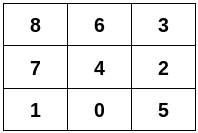
Input: n = 9, edges = [[0,1],[0,4],[0,5],[1,7],[2,3],[2,4],[2,5],[3,6],[4,6],[4,7],[6,8],[7,8]]
Output: [[8,6,3],[7,4,2],[1,0,5]]
Explanation:
Constraints:
2 <= n <= 5 * 1041 <= edges.length <= 105edges[i] = [ui, vi]0 <= ui < vi < nedges can form a 2D grid that satisfies the conditions.Problem Overview: You are given an undirected graph that represents a valid grid structure. The goal is to place every node into a 2D matrix so that graph edges match the four grid neighbors (up, down, left, right). The layout must reconstruct the original grid shape while preserving adjacency.
Approach 1: Degree-Based Row Construction + BFS Placement (O(V + E) time, O(V) space)
The key observation is that nodes in a grid have predictable degrees. Corners have degree 2, edge cells have degree 3, and internal cells have degree 4. Start by identifying a corner node (degree 2). From that corner, walk through neighbors that also belong to the boundary to construct the first row of the grid. Once the top row is fixed, run a BFS traversal from these nodes to fill the remaining rows. Maintain a visited set and adjacency list from the graph. Each BFS expansion places neighbors directly below their corresponding parent cell, ensuring adjacency matches the original edges. This approach works because the graph guarantees a valid grid layout, so every node has a deterministic position relative to previously placed nodes.
Approach 2: Coordinate Assignment with BFS Traversal (O(V + E) time, O(V) space)
Another practical approach assigns coordinates while performing a single BFS. Pick any corner node as the origin and give it coordinate (0,0). As you traverse neighbors, assign them adjacent coordinates such as (x+1,y), (x-1,y), (x,y+1), or (x,y-1). A hash map stores the coordinate of each node and prevents revisiting. Because the input graph forms a valid grid, coordinate conflicts will not occur. After BFS finishes, normalize the coordinates so the smallest row and column start at zero, then place nodes into a matrix. This technique treats the grid reconstruction as a coordinate labeling problem over a breadth-first search traversal.
Recommended for interviews: The BFS coordinate assignment approach is usually the cleanest explanation. It shows you understand graph traversal and spatial reconstruction. Mentioning node-degree properties demonstrates deeper insight about grid graphs, but BFS placement is typically what interviewers expect because it directly maps graph neighbors to grid coordinates in linear time.
| Approach | Time | Space | When to Use |
|---|---|---|---|
| Degree-Based Row Construction + BFS | O(V + E) | O(V) | When you want deterministic grid reconstruction using node degree properties |
| BFS Coordinate Assignment | O(V + E) | O(V) | General case; simplest implementation that maps neighbors to coordinates |
| Brute Force Placement with Adjacency Validation | O(V^2) | O(V) | Useful only for understanding the constraint; impractical for large graphs |