Watch 5 video solutions for Best Position for a Service Centre, a hard level problem involving Array, Math, Geometry. This walkthrough by Programming Live with Larry has 1,934 views views. Want to try solving it yourself? Practice on FleetCode or read the detailed text solution.
A delivery company wants to build a new service center in a new city. The company knows the positions of all the customers in this city on a 2D-Map and wants to build the new center in a position such that the sum of the euclidean distances to all customers is minimum.
Given an array positions where positions[i] = [xi, yi] is the position of the ith customer on the map, return the minimum sum of the euclidean distances to all customers.
In other words, you need to choose the position of the service center [xcentre, ycentre] such that the following formula is minimized:
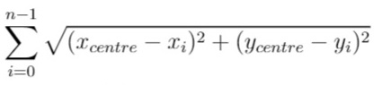
Answers within 10-5 of the actual value will be accepted.
Example 1:
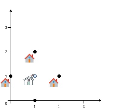
Input: positions = [[0,1],[1,0],[1,2],[2,1]]
Output: 4.00000
Explanation: As shown, you can see that choosing [xcentre, ycentre] = [1, 1] will make the distance to each customer = 1, the sum of all distances is 4 which is the minimum possible we can achieve.
Example 2:
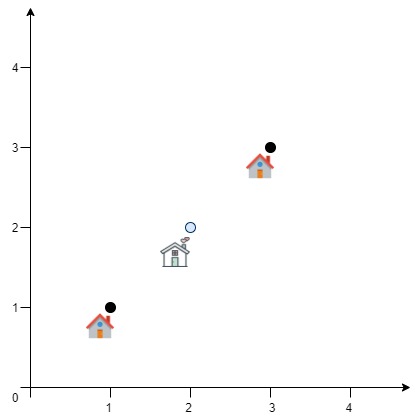
Input: positions = [[1,1],[3,3]]
Output: 2.82843
Explanation: The minimum possible sum of distances = sqrt(2) + sqrt(2) = 2.82843
Constraints:
1 <= positions.length <= 50positions[i].length == 20 <= xi, yi <= 100Problem Overview: You receive several customer coordinates on a 2D plane. The task is to place a service center so that the sum of Euclidean distances from the center to all customers is minimized. Unlike Manhattan-distance problems, the Euclidean metric makes the objective function continuous and non-linear, so typical discrete search strategies do not work directly.
Approach 1: Gradient Descent Optimization (O(n × iterations) time, O(1) space)
The total distance function is continuous across the plane, which allows you to treat the problem as numerical optimization. Start from an initial guess (often the centroid of all points). Compute the gradient of the distance function with respect to x and y, then move the candidate point in the direction that decreases the total distance. After each step, reduce the learning rate to stabilize convergence. Each iteration scans all points and accumulates gradient components, giving O(n) work per step. This approach fits naturally when working with math and geometry optimization problems where the solution lies in continuous space.
The key insight: the minimum occurs where the gradient approaches zero. By repeatedly updating the position using small steps, the algorithm converges toward the geometric median. Precision improves as the step size shrinks. Because the search happens in continuous space rather than over a grid, you avoid exponential brute-force exploration.
Approach 2: Simulated Annealing (O(n × iterations) time, O(1) space)
Simulated annealing treats the coordinate as a candidate solution and randomly explores nearby positions. Start from an initial point (again, the centroid works well). At each step, generate random neighboring positions and compute the change in total distance. If the new position improves the objective, accept it. If it is worse, accept it with a probability controlled by a temperature parameter. Gradually cool the temperature so the search transitions from exploration to exploitation.
This randomized search helps escape local minima and works well for continuous optimization problems. Each candidate evaluation requires summing distances to all points, so the cost per iteration is O(n). The approach connects to randomized algorithms and still relies heavily on geometric distance calculations from the array of coordinates.
Recommended for interviews: Gradient descent is typically preferred. It demonstrates understanding of continuous optimization and geometric median concepts while remaining relatively simple to implement. Simulated annealing is useful when discussing randomized optimization strategies, but interviewers usually expect the deterministic gradient-descent style search. Showing both indicates strong problem-solving depth.
| Approach | Time | Space | When to Use |
|---|---|---|---|
| Gradient Descent Optimization | O(n × iterations) | O(1) | Deterministic continuous optimization; typical interview-friendly solution |
| Simulated Annealing | O(n × iterations) | O(1) | When randomized search helps escape local minima or when discussing probabilistic optimization |