
Shortest Path in a Weighted Tree - Solution & Explanation
Problem Statement
You are given an integer n and an undirected, weighted tree rooted at node 1 with n nodes numbered from 1 to n. This is represented by a 2D array edges of length n - 1, where edges[i] = [ui, vi, wi] indicates an undirected edge from node ui to vi with weight wi.
You are also given a 2D integer array queries of length q, where each queries[i] is either:
[1, u, v, w']– Update the weight of the edge between nodesuandvtow', where(u, v)is guaranteed to be an edge present inedges.[2, x]– Compute the shortest path distance from the root node 1 to nodex.
Return an integer array answer, where answer[i] is the shortest path distance from node 1 to x for the ith query of [2, x].
Example 1:
Input: n = 2, edges = [[1,2,7]], queries = [[2,2],[1,1,2,4],[2,2]]
Output: [7,4]
Explanation:
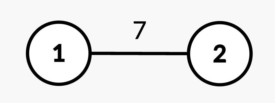
- Query
[2,2]: The shortest path from root node 1 to node 2 is 7. - Query
[1,1,2,4]: The weight of edge(1,2)changes from 7 to 4. - Query
[2,2]: The shortest path from root node 1 to node 2 is 4.
Example 2:
Input: n = 3, edges = [[1,2,2],[1,3,4]], queries = [[2,1],[2,3],[1,1,3,7],[2,2],[2,3]]
Output: [0,4,2,7]
Explanation:
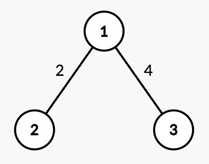
- Query
[2,1]: The shortest path from root node 1 to node 1 is 0. - Query
[2,3]: The shortest path from root node 1 to node 3 is 4. - Query
[1,1,3,7]: The weight of edge(1,3)changes from 4 to 7. - Query
[2,2]: The shortest path from root node 1 to node 2 is 2. - Query
[2,3]: The shortest path from root node 1 to node 3 is 7.
Example 3:
Input: n = 4, edges = [[1,2,2],[2,3,1],[3,4,5]], queries = [[2,4],[2,3],[1,2,3,3],[2,2],[2,3]]
Output: [8,3,2,5]
Explanation:
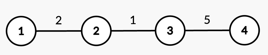
- Query
[2,4]: The shortest path from root node 1 to node 4 consists of edges(1,2),(2,3), and(3,4)with weights2 + 1 + 5 = 8. - Query
[2,3]: The shortest path from root node 1 to node 3 consists of edges(1,2)and(2,3)with weights2 + 1 = 3. - Query
[1,2,3,3]: The weight of edge(2,3)changes from 1 to 3. - Query
[2,2]: The shortest path from root node 1 to node 2 is 2. - Query
[2,3]: The shortest path from root node 1 to node 3 consists of edges(1,2)and(2,3)with updated weights2 + 3 = 5.
Constraints:
1 <= n <= 105edges.length == n - 1edges[i] == [ui, vi, wi]1 <= ui, vi <= n1 <= wi <= 104- The input is generated such that
edgesrepresents a valid tree. 1 <= queries.length == q <= 105queries[i].length == 2or4queries[i] == [1, u, v, w']or,queries[i] == [2, x]1 <= u, v, x <= n(u, v)is always an edge fromedges.1 <= w' <= 104
Approach Overview
Problem Overview: You are given a weighted tree and need to compute the shortest path distance between nodes. Because a tree contains exactly one simple path between any two nodes, the task reduces to efficiently calculating distances along that path, often across many queries.
Approach 1: DFS per Query (Brute Force) (Time: O(n) per query, Space: O(n))
The most direct strategy runs a DFS from the source node until the destination node is reached. While traversing, accumulate edge weights and stop once the target appears. Since a tree has no cycles, the traversal visits each node at most once. This works for a small number of queries but becomes expensive when the query count grows because each query can traverse the entire tree.
Approach 2: Prefix Distance + Lowest Common Ancestor (Time: O(n log n) preprocessing, O(log n) per query, Space: O(n log n))
Precompute the distance from a chosen root to every node using a single DFS. Store dist[node] as the total weight from the root. The distance between two nodes u and v can then be computed using their Lowest Common Ancestor: dist[u] + dist[v] - 2 * dist[lca(u,v)]. LCA queries are answered using binary lifting tables built during preprocessing. This reduces repeated traversal and turns path distance queries into constant arithmetic plus an LCA lookup. See related techniques in Tree and Depth-First Search.
Approach 3: Euler Tour + Binary Indexed Tree / Segment Tree (Time: O((n + q) log n), Space: O(n))
If the problem includes edge weight updates or dynamic queries, combine an Euler tour with a range data structure. Flatten the tree into an array using entry/exit times from DFS. Store edge contributions in a Binary Indexed Tree or Segment Tree. Distance from root to any node becomes a prefix query on the flattened structure, while updates propagate with log n modifications. Path distance queries still use the LCA formula but fetch prefix sums dynamically. This approach appears frequently in advanced tree problems involving updates. See Binary Indexed Tree and Segment Tree.
Recommended for interviews: Start by explaining the DFS brute force to show understanding of tree traversal. Interviewers typically expect the LCA + prefix distance solution because it answers queries in O(log n) after preprocessing. If the problem introduces updates, extending the design with Euler tour and Fenwick/Segment Tree demonstrates strong tree algorithm skills.
Solutions for this problem are being prepared.
Try solving it yourselfDetailed Complexity Analysis
| Approach | Time | Space | When to Use |
|---|---|---|---|
| DFS per Query | O(n) per query | O(n) | Small trees or very few queries |
| Prefix Distance + LCA (Binary Lifting) | O(n log n) preprocessing, O(log n) query | O(n log n) | Standard solution for many shortest path queries in a static tree |
| Euler Tour + Fenwick / Segment Tree | O((n + q) log n) | O(n) | When edge weights can change or queries require dynamic updates |
Video Solution
L-9. Shortest Path In a Weighted Tree • Segment Tree Series • Leetcode Biweekly 154 Contest • ET+LP • Why Not DP [By Piyush Raj] • 661 views views
Watch 2 more video solutions →Frequently Asked Questions
Is Shortest Path in a Weighted Tree easy or hard?
Shortest Path in a Weighted Tree Python/Java solution
How to solve Shortest Path in a Weighted Tree in O(n)?
What is the best approach for Shortest Path in a Weighted Tree?
Is Shortest Path in a Weighted Tree asked at Google/Amazon/Meta?
What data structure is used in Shortest Path in a Weighted Tree?
What is the time complexity of Shortest Path in a Weighted Tree?
Ready to solve this problem?
Practice Shortest Path in a Weighted Tree with our built-in code editor and test cases.
Practice on FleetCode